22 September 2026 · activation-functionsrelugeluml-foundation
Activation functions roadmap: step, sigmoid, tanh, ReLU, Leaky ReLU, GELU
An activation function is the small non-linear function each neuron applies to its output. This post goes through the common ones in the order they were invented, what each fixed, what each broke, and how to write every one in PyTorch.
Stack ten layers of a neural network with nothing between them and the result can only draw straight-line boundaries, no matter how deep it is. The small function each neuron applies to its output before passing it on is what removes that limit, and it is called an activation function. Pick the wrong one and a deep network stops learning. Below are the six you will meet, in the order they were invented, because each one fixes a problem in the one before it.
How a neuron applies it
A neuron multiplies its inputs $\mathbf{x}$ by weights $\mathbf{w}$, adds a bias $b$, and gets one number $z$. The activation $f$ turns $z$ into the output $a$:
$$a = f(z), \qquad z = \mathbf{w} \cdot \mathbf{x} + b$$
In PyTorch this is the nn.ReLU() line between two nn.Linear layers.
Why a network needs one
A layer with no activation computes $\mathbf{W}\mathbf{x} + \mathbf{b}$, a multiply by a matrix and then an add. A function built only from multiplies and adds like that is called linear, and a linear function can only split its input with a straight line. Feed one linear function into another and the result is still one multiply and one add, so ten stacked linear layers collapse into a single one with the same straight-line limit. The activation $f$ is chosen to be non-linear, a function whose graph bends, and one non-linear step between the layers stops the collapse. The network can then learn curved boundaries.
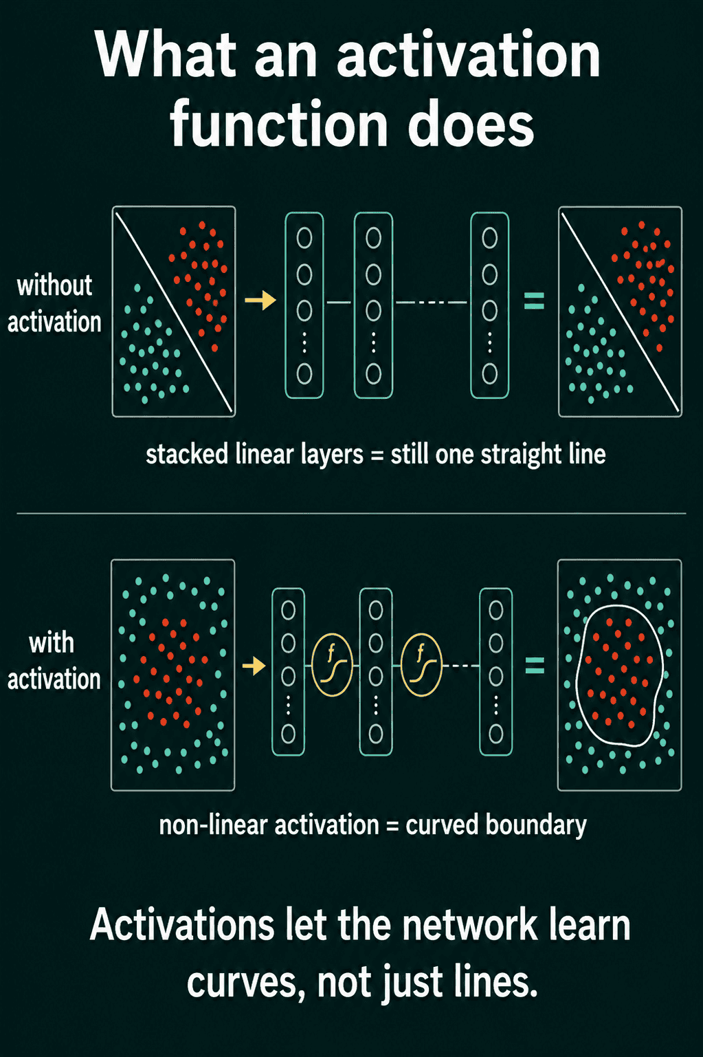
So the question is which $f$ to use, and the rest of this post is the history of that answer.
The step function: non-linear but untrainable
The earliest choice, used by the perceptron, outputs 1 for positive inputs and 0 for everything else:
$$f(z) = \begin{cases} 1 & z > 0 \\ 0 & z \le 0 \end{cases}$$
It is non-linear, but gradient descent cannot train through it. Training works by asking how a tiny change in a weight changes the loss, and that answer flows backward through each activation's slope. The step function's slope is 0 everywhere except at $z = 0$, where it jumps, so the answer is always "no change" and no weight ever moves.
1import torch
2
3def step(z):
4    return (z > 0).float()
5
6# PyTorch has torch.heaviside, but no nn layer wraps it: nothing trains through it
Sigmoid: trainable but vanishing
Sigmoid squashes $z$ smoothly into the range between 0 and 1:
$$\sigma(z) = \frac{1}{1 + e^{-z}}$$
Its slope is $\sigma(z)(1 - \sigma(z))$, which peaks at $0.25$ when $z = 0$ and shrinks toward 0 as $z$ moves away from 0 in either direction. That shrinking is the problem. The gradient reaching an early layer is the product of the slopes of every activation it passed through. Through 9 sigmoid layers the best case is $0.25^9$, about $4 \times 10^{-6}$, and in a real network most neurons sit far from $z = 0$ where the slope is much smaller still. The early layers receive almost no gradient and stop learning. This is the vanishing gradient problem, and sigmoid causes it badly.
1def sigmoid(z):
2    return 1 / (1 + torch.exp(-z))
3
4torch.nn.Sigmoid()  # fine as an output layer, avoid in hidden layers
Tanh: zero-centred, still saturates
Tanh is the same S shape rescaled to run from -1 to 1:
$$\tanh(z) = \frac{e^{z} - e^{-z}}{e^{z} + e^{-z}}$$
Two things improve. Its outputs are centred on 0, so the weight gradients inside a layer can have mixed signs instead of all pushing the same way, and its maximum slope is 1 instead of $0.25$. It still flattens out for large positive or negative $z$, so in a deep stack saturated neurons still pass tiny gradients. Tanh survives today mostly inside the gates of recurrent networks.
1def tanh(z):
2    e_pos, e_neg = torch.exp(z), torch.exp(-z)
3    return (e_pos - e_neg) / (e_pos + e_neg)
4
5torch.nn.Tanh()
ReLU: the one that made deep networks train
ReLU keeps positive inputs unchanged and sets negative ones to 0:
$$f(z) = \max(0, z)$$
For any $z > 0$ the slope is exactly 1, so the gradient passes through unchanged no matter how deep the network is. It is also a single comparison, far cheaper than an exponential, and roughly half of the neurons output 0 on any given input, which keeps the computation sparse. This is why ReLU is the default hidden-layer activation for most feedforward and convolutional networks.
The cost is the other side of zero. For $z \le 0$ the slope is 0, so a neuron whose $z$ is negative on every training example gets no gradient, never updates, and stays at 0 for good. These are called dead neurons.
1def relu(z):
2    return torch.clamp(z, min=0)   # or torch.maximum(z, torch.zeros_like(z))
3
4torch.nn.ReLU()
Leaky ReLU: a small slope for dead neurons
Leaky ReLU gives the negative side a small slope $\alpha$, usually $0.01$, instead of 0:
$$f(z) = \begin{cases} z & z > 0 \\ \alpha z & z \le 0 \end{cases}$$
A neuron on the wrong side of zero now receives a small gradient and can recover. The price is one extra hyperparameter, and in practice $\alpha = 0.01$ works in most setups. Reach for it when you measure a large fraction of units outputting exactly 0 across the dataset and better weight initialisation has not helped.
1def leaky_relu(z, alpha=0.01):
2    return torch.where(z > 0, z, alpha * z)
3
4torch.nn.LeakyReLU(negative_slope=0.01)
GELU: the transformer default
GELU multiplies $z$ by the probability that a standard normal random draw is below $z$, written $\Phi(z)$:
$$\text{GELU}(z) = z \cdot \Phi(z)$$
For large positive $z$ that probability is close to 1 and GELU behaves like $z$; for large negative $z$ it is close to 0 and GELU behaves like 0. Near zero it bends smoothly instead of ReLU's hard corner, and it dips slightly below 0 before rising. Transformers adopted it and it is the standard activation in their feedforward blocks. On language tasks it usually matches or beats ReLU by a small margin.
1import math
2
3def gelu(z):
4    return 0.5 * z * (1 + torch.erf(z / math.sqrt(2)))
5
6torch.nn.GELU()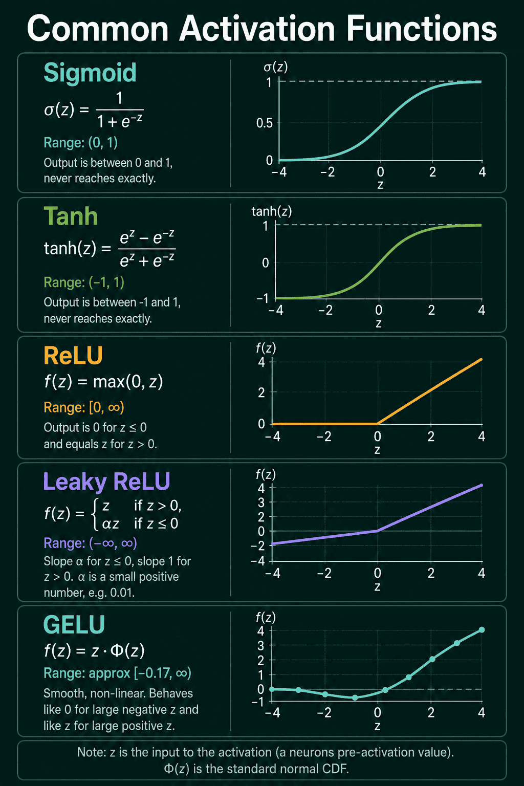
Other activations you will see
Most newer activations are variations on the same two goals: keep gradients alive and avoid dead units. ELU gives the negative side a smooth exponential tail. SELU is ELU scaled so that, under specific initialisation and architecture conditions, layer outputs keep a fixed mean and variance. Mish is smooth and dips below zero like GELU, and shows up in some vision models. SiLU, also called Swish, is $z \cdot \sigma(z)$, close in shape to GELU, and the gated variants built on it (SwiGLU, GeGLU) are what many current large language models use. PyTorch has nn.ELU(), nn.SELU(), nn.Mish(), and nn.SiLU() for all four.
Output activations are a separate question
Everything above is about hidden layers. The output layer's activation is set by the loss, not by training dynamics. Sigmoid on a single output gives a probability for binary classification, softmax across the outputs gives a probability per class for multiclass, and regression uses no activation at all. In PyTorch you usually leave the output activation out of the model: BCEWithLogitsLoss applies the sigmoid and CrossEntropyLoss applies the softmax internally, which is more numerically stable than doing it yourself.
Which one to use
| Where | Use |
|---|---|
| Hidden layers, default | nn.ReLU() |
| Transformer feedforward blocks | nn.GELU() |
| Many dead neurons measured | nn.LeakyReLU() |
| Binary output | sigmoid, inside BCEWithLogitsLoss |
| Multiclass output | softmax, inside CrossEntropyLoss |
| Regression output | none |
Two mistakes come up often. The first is sigmoid or tanh in the hidden layers of a deep network, which usually shows up as a loss that barely moves. The second is putting nn.Softmax at the end of a model and then passing that into CrossEntropyLoss, which applies softmax a second time and trains slower than it should.
QuiddityML teaches each of these activations as its own concept in the ML Foundation track, in this same order, and the exercises on them include writing sigmoid, ReLU, and GELU from scratch, spotting a sigmoid hiding in a deep hidden layer, and checking a layer for dead units.
Related concepts
The vanishing gradient problem is the reason sigmoid and tanh fell out of hidden layers, and residual connections are the other main fix for it in very deep networks. Weight initialisation decides how many neurons start dead under ReLU, which is why Kaiming initialisation is paired with it. Batch normalisation and layer normalisation keep $z$ in the range where these activations have useful slopes.