15 September 2026 · optimizersml-foundation

What is the Adam optimizer? Explained step by step

Adam is the optimizer most deep learning models train with. This post explains what it does, why it works better than plain gradient descent, and when to use AdamW instead.

Adam is an algorithm that decides how much to change each parameter of a model after every training step. Almost every deep learning model you have heard of was trained with it or with its close relative AdamW. Most people write torch.optim.Adam(model.parameters(), lr=1e-3) and move on, which works until training blows up and they have no idea which knob to turn. This post explains what Adam does and why, with no background needed beyond knowing that a model has parameters that get trained.

What an optimizer does

Training a model means repeating one loop: make a prediction, measure how wrong it was (the loss), compute for each parameter which direction would reduce the loss (the gradient), and move each parameter a little in that direction. The optimizer is the part that decides how big "a little" is, for each parameter, on each step.

The simplest optimizer is gradient descent: multiply the gradient by one fixed number, the learning rate, and subtract it from the parameter. Every parameter gets the same learning rate, and every step looks only at the current gradient.

The problem Adam solves

Plain gradient descent has two weaknesses.

It has no memory. Each step follows the current gradient alone. If the gradient points left on one step and right on the next, the parameter zigzags instead of making progress.

It uses one learning rate for everything. Some parameters get tiny gradients and barely move; others get huge gradients and overshoot. One number cannot be right for both.

Two older fixes address these separately. Momentum keeps a running average of past gradients, so consistent directions build up speed and zigzags cancel out. RMSProp keeps a running average of how large each parameter's gradients have been, and gives parameters with large gradients smaller steps and parameters with small gradients larger steps. Adam does both at once, which is why the name stands for "adaptive moment estimation".

What Adam keeps in memory

For every parameter, Adam stores two numbers that it updates on every step.

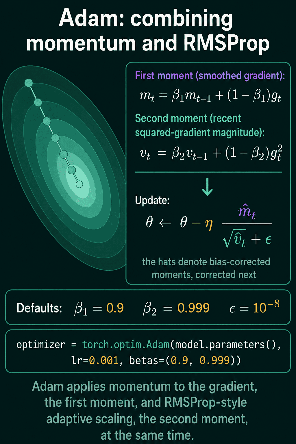
The first is a running average of the gradient itself. Call it $m$. It remembers which direction the gradient has mostly been pointing. This is the momentum part.

The second is a running average of the gradient squared. Call it $v$. Squaring throws away the sign, so $v$ only remembers how large the gradients have been, not their direction. This is the RMSProp part.

Both are "exponential moving averages": on each step, keep most of the old value and blend in a little of the new gradient. Two constants control how much is kept. $\beta_1$ (beta one) is for $m$ and defaults to 0.9, meaning 90% old, 10% new. $\beta_2$ (beta two) is for $v$ and defaults to 0.999, meaning it changes very slowly. With $g$ as the current gradient and $t$ as the step number:

$$m_t = \beta_1 m_{t-1} + (1-\beta_1) g_t$$

$$v_t = \beta_2 v_{t-1} + (1-\beta_2) g_t^2$$

The update rule

Adam moves each parameter by the smoothed direction divided by the square root of the smoothed size. With $\theta$ (theta) as the parameter and $\eta$ (eta) as the learning rate:

$$\theta \leftarrow \theta - \eta \frac{m_t}{\sqrt{v_t} + \epsilon}$$

The square root brings $v$ back to the same units as the gradient, since $v$ was built from squared gradients. $\epsilon$ (epsilon, default $10^{-8}$) is a tiny constant that stops division by zero when $v$ is nearly zero.

Read the fraction as "direction divided by typical size". A parameter whose gradients have been consistently large gets a smaller step, because the denominator is large. A parameter whose gradients have been small gets a larger step. Every parameter ends up moving by roughly the same amount per step, regardless of how big its raw gradients are. That is what makes Adam forgiving about the learning rate: 1e-3 works for a surprising range of models.

The bias correction, or why the real formula has hats

Both $m$ and $v$ start at zero. On the first step, $m$ is 10% of the gradient and $v$ is 0.1% of the gradient squared, because the averages have not seen enough history yet. Both are far too small, but $v$ is much more too small than $m$, because $\beta_2$ is closer to 1. Dividing a slightly-too-small $m$ by the square root of a badly-too-small $v$ gives an update that is several times too large. Early Adam steps would be wild.

The fix is to divide each average by how much history it has actually accumulated:

$$\hat m_t = \frac{m_t}{1-\beta_1^t}, \qquad \hat v_t = \frac{v_t}{1-\beta_2^t}$$

The hat means "corrected". At step 1, $m$ is scaled up by 10 and $v$ by 1000, which puts them back at the size they would have if they had a full history. As $t$ grows, $\beta^t$ shrinks toward zero, the denominators approach 1, and the correction fades out. The real Adam update uses $\hat m$ and $\hat v$ in place of $m$ and $v$.

The correction fixes the systematic error. It does not fix noise: at step 5, $\hat v$ is the right size on average but was built from only five gradients, so early updates are still bumpier than later ones.

In code

import torch

optimizer = torch.optim.Adam(model.parameters(), lr=1e-3, betas=(0.9, 0.999), eps=1e-8)

for batch in loader:
    optimizer.zero_grad()
    loss = loss_fn(model(batch.x), batch.y)
    loss.backward()
    optimizer.step()

If training diverges in the first few hundred steps, lower the learning rate first (try 3e-4). If it trains but plateaus early, the learning rate is usually too low. Leave the betas alone unless you have a specific reason.

When to use AdamW instead

Weight decay is a common regularization trick: on every step, shrink each parameter slightly toward zero so the model does not rely on any one weight too much. The traditional way to do this is to add a decay term to the gradient before the optimizer sees it.

With Adam that goes wrong. Adam divides everything in the gradient by $\sqrt{\hat v}$, including the decay term, so parameters with large historical gradients get less decay than you asked for. The regularization becomes uneven in a way you did not choose.

AdamW applies the decay as its own separate step, outside the adaptive scaling, with $\lambda$ (lambda) as the decay strength:

$$\theta \leftarrow \theta - \eta \frac{\hat m_t}{\sqrt{\hat v_t} + \epsilon} - \eta \lambda \theta$$

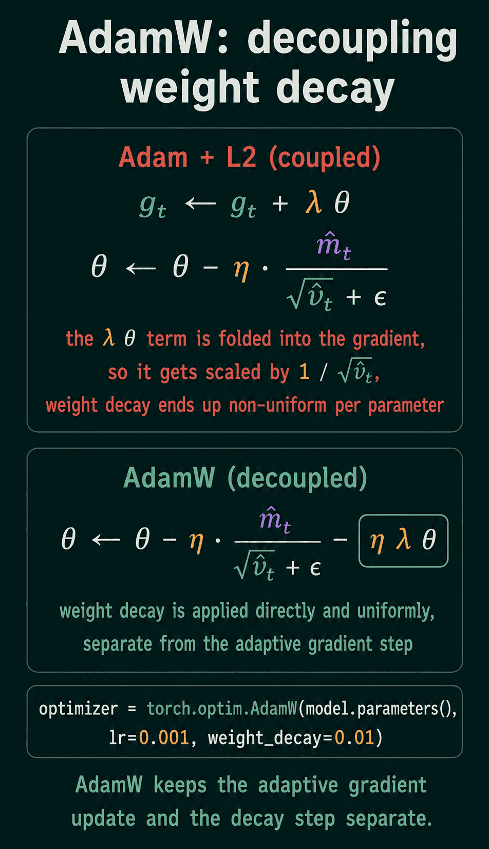
The gradient part stays adaptive and the decay stays uniform. If you want weight decay with Adam, use AdamW. Most transformer training recipes do.

optimizer = torch.optim.AdamW(model.parameters(), lr=1e-3, weight_decay=0.01)

Adam, SGD, and the others in one paragraph

SGD with momentum is Adam without the per-parameter scaling; it is simpler, and for image classification with careful learning rate schedules it sometimes generalizes slightly better, but it needs more tuning. RMSProp is Adam without momentum and without bias correction. Adam is the default when you want something that works on the first try. AdamW is Adam with weight decay done correctly, and is the default for transformers and most modern models.

Common mistakes

Using Adam with L2 regularization added to the loss and expecting it to behave like weight decay; use AdamW. Cranking the learning rate to 1e-2 because "Adam is adaptive"; the scaling helps, but 1e-3 or lower is still where most models live. Forgetting optimizer.zero_grad(), which makes gradients accumulate across steps and looks like the optimizer is broken.

QuiddityML's ML Foundation track covers gradient descent, momentum, RMSProp, Adam, and AdamW as separate concepts with exercises on each, at quiddityml.com.