22 September 2026 · bias-varianceoverfittinggeneralizationml-foundation
Bias-variance tradeoff explained with pictures
A model can be wrong on new data in two different ways, and the fixes for each pull in opposite directions. This post shows both with plots, how to tell them apart from your training and validation loss, and what to change for each.
A model that fits its training data well can still be wrong on new data, and it can be wrong in two different ways. It can be too simple to follow the real pattern at all, or it can follow the training points so closely that it also follows the noise in them. The first kind of error is called bias and the second is called variance. Shrinking one usually grows the other, which is why the pair is called the bias-variance tradeoff. The reason to care is that the fix for each one makes the other worse, so guessing wrong about which you have sends you in the wrong direction.
Error on new data is the number that matters
The training set is the examples the model updates its parameters on. A held-out set, usually called the validation set, is examples the model never trains on, kept aside to measure how well what it learned carries over. A model can score well on training data by memorizing it, so the held-out score is the one that says whether the model works. Bias and variance are two reasons that held-out score can be bad.
What bias is
Bias is error that comes from a model too simple to represent the pattern in the data. The picture to hold in mind is a set of points that trace an arch, and a straight horizontal line fitted through them. The line sits at the average height, misses the top of the arch and both ends, and no amount of extra training data moves it, because a straight line cannot bend. A model with high bias is wrong in the same direction on every training set, and the usual word for that state is underfitting.
What variance is
Variance is error that comes from a model sensitive to which particular examples it happened to train on. The same arch of points, fitted this time by a curve with far more parameters than it needs, comes out as a jagged line that passes through every point, including the ones that sit off the arch because of measurement noise. Train that same model on a second sample of points from the same arch and the jagged line lands somewhere else. The model is not learning the arch, it is learning the sample, and the usual word for that state is overfitting.
The fit that sits between them
Between the flat line and the jagged one is a smooth curve that follows the arch and ignores the scatter around it. It has enough capacity to bend but not enough to chase individual points. Its error on new data is lower than either extreme, and finding it is the practical goal.
The three fits can be put on one axis. Model complexity means how many parameters a model has, or how many ways it can bend, so the horizontal line, the smooth curve, and the jagged curve sit left to right on a complexity axis. Along that axis, bias falls as complexity grows, because a more flexible model can follow more of the pattern, while variance rises, because a more flexible model can also follow more of the noise. The error on new data is the sum of the two plus a floor no model can remove, and that sum traces a U shape: high on the left from bias, high on the right from variance, and lowest somewhere in between.
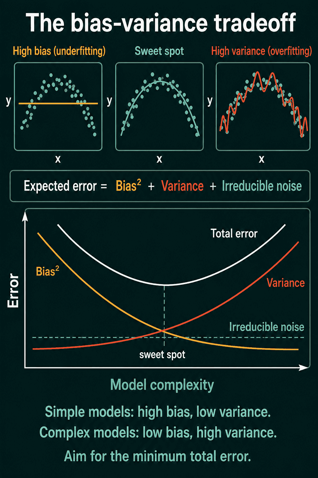
The equation
The error floor is called irreducible noise, and it is the randomness in the labels themselves, such as measurement error, which no model can predict. For squared-error loss, the expected error of a model on a new input splits exactly into three pieces:
$$\text{Expected error} = \text{Bias}^2 + \text{Variance} + \text{Irreducible noise}$$
Bias enters squared because it is a signed distance and the loss is squared. The equation says total error is bias and variance added together, so lowering one only helps if the other does not rise by more.
In words, bias is how far the average of the models you would get across many different training sets sits from the true relationship, and variance is how much any single one of those models moves away from that average when the training set changes. The split is exact for squared error and a useful approximation for other losses such as cross-entropy.
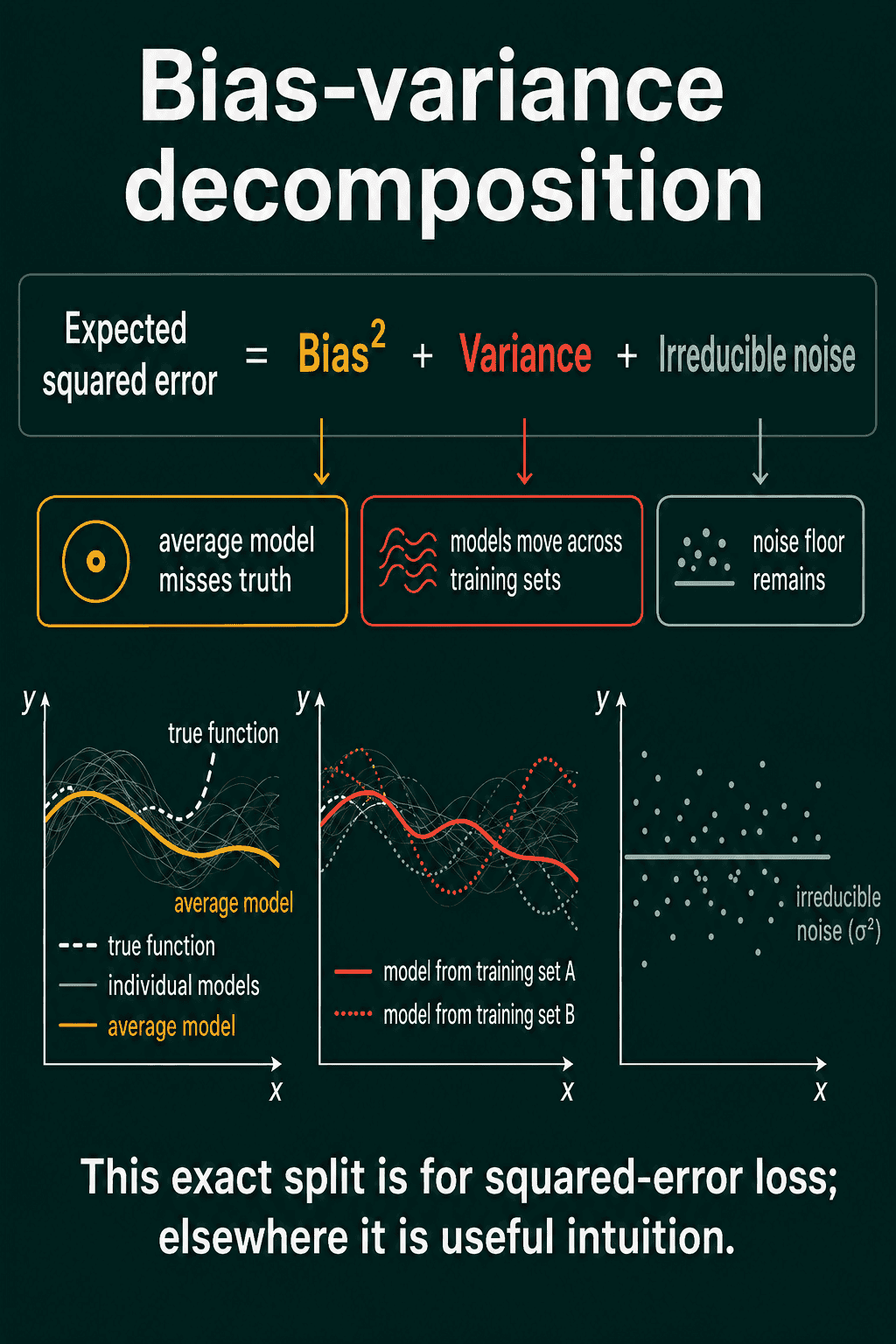
How to tell which one you have
Retraining on many training sets and averaging is not something you get to do in practice, so the diagnosis comes from two numbers you already have: the loss on the training set and the loss on the validation set, tracked over the course of training.
| Training loss | Validation loss | Diagnosis |
|---|---|---|
| high | high, close to training | high bias, underfitting |
| low | high, gap growing | high variance, overfitting |
| low | low, small gap | close to the sweet spot |
The gap between the two curves is the variance signal, and the height of the training curve is the bias signal. A model that cannot even fit its training data is not memorizing anything, so both losses sit high together. A model that memorizes drives training loss down while validation loss stalls or climbs.
What to change for bias
High bias means the model needs more room to bend. The usual moves are a wider or deeper network, more training epochs, a higher learning rate if the loss was still dropping when training stopped, extra input features that carry signal, and less regularization. Regularization is the set of techniques that hold a model back from fitting too closely, such as weight decay and dropout, and turned up too far it blocks fitting altogether.
What to change for variance
High variance means the model has more freedom than the data can pin down. The usual moves are more training data, weight decay, dropout, early stopping, and a smaller network. Each of these accepts a small rise in bias to buy a larger drop in variance, and the picture below is what that trade looks like in the error budget.
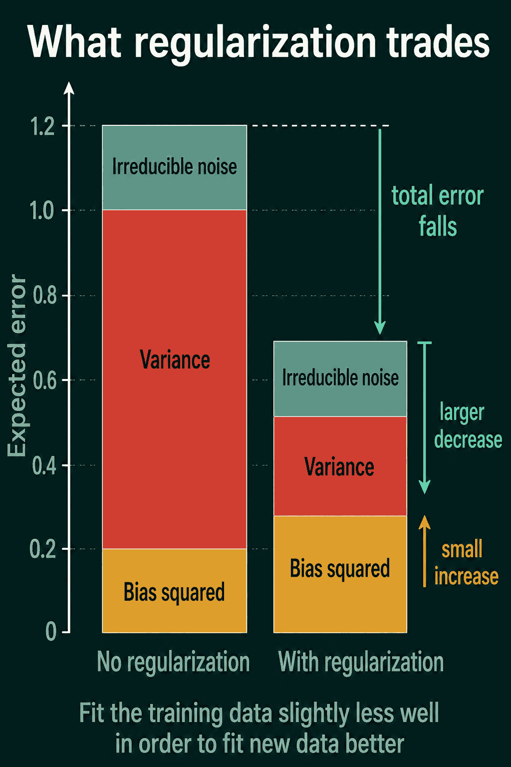
Code
The snippet fits a tiny network and a large one to the same noisy sine curve and prints both losses for each. The small model lands with both losses high, and the large one drives training loss low while validation loss stays higher.
1import torch
2import torch.nn as nn
3
4torch.manual_seed(0)
5x = torch.linspace(-3, 3, 200).unsqueeze(1)
6y = torch.sin(x) + 0.3 * torch.randn_like(x)      # true curve plus noise
7x_train, y_train = x[::2], y[::2]                 # even rows train
8x_val, y_val = x[1::2], y[1::2]                   # odd rows validate
9
10def fit(hidden, epochs=3000):
11    model = nn.Sequential(nn.Linear(1, hidden), nn.Tanh(), nn.Linear(hidden, 1))
12    opt = torch.optim.Adam(model.parameters(), lr=1e-2)
13    for _ in range(epochs):
14        opt.zero_grad()
15        loss = nn.functional.mse_loss(model(x_train), y_train)
16        loss.backward()
17        opt.step()
18    with torch.no_grad():
19        return (nn.functional.mse_loss(model(x_train), y_train).item(),
20                nn.functional.mse_loss(model(x_val), y_val).item())
21
22for hidden in (1, 8, 512):
23    train_loss, val_loss = fit(hidden)
24    print(f"hidden={hidden:4d}  train={train_loss:.3f}  val={val_loss:.3f}")
Validation loss cannot go below the noise in the labels, and the middle width should get closest to that floor. If the large model does not overfit on your run, cut the training set to a few dozen points and the gap opens up.
Common mistakes
Reading training loss alone. A falling training curve says nothing about which side of the U you are on, and the validation curve is the one that carries the variance signal.
Regularizing an underfit model. Adding dropout or weight decay to a model whose training loss is already high pushes it further left on the U-curve, and the right first move is more capacity.
Tuning on the test set. Once a model has been chosen because it scored well on a held-out set, that set no longer measures generalization, so decisions go on the validation set and the test set is used once at the end.
Treating "smaller model" as the automatic fix. Past the point where a model can fit its training data exactly, test error can drop again as the model keeps growing. This is called double descent, and it means the U-curve describes the classic regime and not the whole picture.
Related concepts
Overfitting and underfitting are the same two failures described by what the loss curves do rather than by where the error comes from, and the diagnosis table above is the bridge between the two framings. Regularization is the family of fixes for the variance side, and weight decay, dropout, and early stopping each have enough detail for their own post. Cross-validation rotates which slice of the data is held out, so the validation number does not depend on one particular split, which matters most on small datasets.
QuiddityML teaches the bias-variance tradeoff as its own concept in the ML Foundation track, right after loss curves and before regularization, and its exercises show a pair of loss curves and ask which side of the tradeoff they sit on, then ask which fix moves the model toward the middle.