15 September 2026 · roadmaplearningml-foundation

How to learn machine learning in 2026: a complete roadmap for self-taught learners

The order to learn machine learning on your own: Python, the math that ML uses, PyTorch, then training and evaluating deep networks, with every concept named so you know exactly what is ahead of you.

Machine learning is the practice of fitting a model to data so it makes useful predictions on data it has not seen, and learning it on your own is mostly a problem of order. The material is not secret. It is spread across courses, textbooks, papers, and blog posts, and a common reason people stall is that they hit a concept that quietly assumed three others they skipped. This post is the order. It names every concept you need before your first serious model, grouped into four stages, so you can see what is ahead and check off what you already have.

The four stages are Python, the math that ML actually uses, PyTorch, and the ML foundations themselves. After that you pick a direction. The concept lists below are the ones QuiddityML teaches, in the same order, so if you want the version with lessons, hands-on exercises, and spaced repetition, it is there. If you would rather assemble it yourself from free sources, this list is still the map.

A note on time. Estimates below assume 8 to 10 focused hours a week and that you do exercises, not just reading. Reading alone is faster, and much less of it sticks.

Stage 1: Python (3 to 5 weeks)

You need Python because every ML library, tutorial, and job posting assumes it, and you need a specific slice of it: the parts that show up in data loading, model code, and debugging. Web frameworks, async, and metaprogramming can wait until a project needs them.

The order that works, unit by unit:

1. Getting started: why Python for ML, running it, choosing an editor, syntax basics.
2. Environments: installing Python, virtual environments, package managers, project layout and imports. Many "it works on my machine" problems in ML are environment problems.
3. Variables and objects: numbers, booleans and None, comparisons.
4. Strings: literals, indexing and slicing, immutability, string methods, f-strings.
5. Lists: basics, changing lists, nesting and copying. Copying is where beginners get bitten.
6. Tuples and sets.
7. Dictionaries: basics, safe access and iteration, nested dicts and comprehensions. Model configs and checkpoints are dictionaries.
8. Control flow: conditionals, loops, loop helpers like enumerate and zip.
9. Comprehensions, iterables, iterators, generators. Data pipelines are built out of these.
10. Functions: defining them, flexible signatures with *args and **kwargs, scope and its pitfalls, lambdas.
11. Type hints: reading them and the common shapes. Library docs are written in them.
12. Classes: why classes exist, defining one, inheritance, dunder methods, dataclasses and method decorators. Every PyTorch model is a class that inherits from nn.Module.
13. Errors: exceptions, reading a traceback, handling exceptions, context managers.
14. Files and data I/O: reading and writing files, paths with pathlib, structured data like JSON and CSV.
15. Modules and the standard library: imports, scripts as modules, the standard library you will use, and a map of the ML ecosystem (NumPy, pandas, scikit-learn, PyTorch).
16. Pythonic patterns for ML: decorators as a reader, dynamic attribute access, everyday idioms, debugging habits.

You can move on when you can read a 200-line training script from a GitHub repo and say what each line does.

Stage 2: The math ML actually uses (6 to 10 weeks)

The question people ask most is how much math they need. The pieces below cover what most ML work needs, and proving theorems is not one of them. You need to read an equation in a paper or a docstring and know what it is doing, and you need to know why training breaks when it does, which is usually a math reason.

Six sub-tracks, in this order.

Mathematical toolkit (1 week). This is notation, and skipping it is why equations look scary. Functions, composition and inverses. Exponents and logarithms. Trig functions and the unit circle. Summation and product notation. Argmin and argmax. Hat, tilde, and bar notation. The update arrow. Set membership and shape notation. Combinatorics. Big-O notation.

Linear algebra (3 weeks). Most models are matrix multiplication with something nonlinear in between. Unit 1: scalars, vectors and matrices; span, basis and linear independence; collinearity; matrix multiplication as a linear map; transpose, outer products and other views of matrix multiplication; the Hadamard product; identity, diagonal and symmetric matrices. Unit 2: systems of linear equations and Gaussian elimination; determinant; inverse and singular matrices; rank, column space and null space; trace. Unit 3: the dot product; norms, lengths and distances; angles and cosine similarity; cross product; orthogonality and orthogonal matrices; invariance and equivariance; orthogonal projections; orthonormal basis; least squares. Unit 4: eigenvalues and eigenvectors; change of basis; eigendecomposition; positive semi-definite matrices; Rayleigh quotient and condition number; singular value decomposition; low-rank approximation; QR and Cholesky factorizations. Unit 5: tensors and tensor operations; broadcasting; einsum notation.

Calculus and optimization (2 weeks). Training is calculus: the gradient says which way to move each parameter. Unit 1: limits and continuity; derivatives; partial derivatives; gradients; the Jacobian; the chain rule; matrix calculus; backpropagation through a linear layer; automatic differentiation. Unit 2: the Hessian; Taylor expansion and linearization; convex functions and sets; critical points; local minima and saddle points; definiteness and the eigenvalue test.

Probability and statistics (3 weeks). A loss function is a probabilistic assumption in disguise, and evaluation is statistics. Unit 1: random variables and distributions; PMF vs PDF; dependent and independent variables; joint, marginal and conditional probability; sum and product rules; the union bound; independence; the chain rule of probability; Bayes' theorem. Unit 2: Bernoulli and binomial; Poisson; continuous distributions; the Gaussian; Beta; degrees of freedom; kernel density estimation; the CDF; percentiles; the exponential family. Unit 3: expectation, variance and moments; covariance and correlation; conditional expectation; the multivariate Gaussian and covariance matrices; Mahalanobis distance. Unit 4: the law of large numbers; the central limit theorem; standard error and confidence intervals; hypothesis tests and p-values. Unit 5: maximum likelihood estimation; maximum a posteriori estimation; Bayesian inference; priors and posteriors; the posterior predictive; conjugate priors; bias and variance of an estimator. Unit 6: Monte Carlo estimation; importance sampling; rejection sampling; Markov chain Monte Carlo; the reparameterization trick; bootstrap resampling.

Information theory (3 days). This is where cross-entropy comes from. Self-information, entropy, differential entropy, the maximum entropy principle, cross-entropy, KL divergence, mutual information.

Numerical computation (2 days). Why your loss turned into NaN. Floating-point representation, overflow and underflow in exponentials, the log-sum-exp trick, the exponential moving average.

You can move on when you can read the softmax cross-entropy loss as an equation and say why it is written with logs.

Stage 3: PyTorch (2 weeks)

Learn the tensor library before you learn models, because most model bugs turn out to be tensor bugs: a wrong shape, a wrong dtype, a view that was secretly a copy, a gradient that did not flow.

Unit 1: what PyTorch is; what a tensor is; creating tensors; tensor datatypes; tensor attributes; storage and layout; views and copies; reshaping; indexing and joining; a first look at autograd. Unit 2: operating on tensors; elementwise math; broadcasting; matrix multiplication; reduction; comparison and selection. Unit 3: PyTorch and NumPy; reproducibility and random number generators; devices; serialization; utilities and housekeeping.

You can move on when you can take a tensor of shape (batch, seq, features), describe what every dimension holds, and reshape it without guessing.

Stage 4: ML foundations (10 to 14 weeks)

This is the core and it is the longest stage on purpose. Deep learning specializations build on these five units, and a lot of what goes wrong in practice is one of these concepts misunderstood. One line per concept, in teaching order.

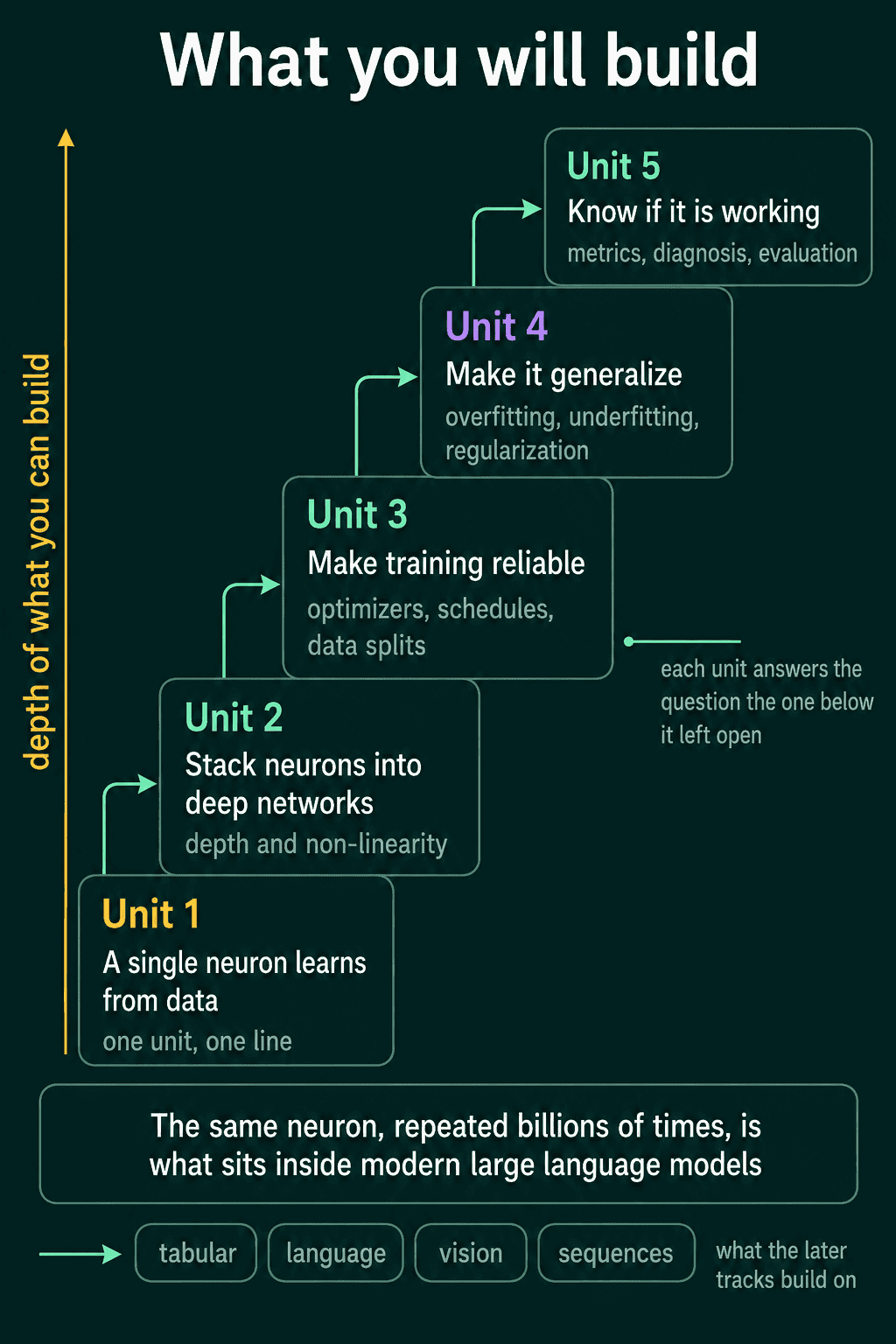
Unit 1: From one neuron to a classifier

• How machines learn: a model, a loss, and a rule for changing the model to reduce the loss.
• The ML taxonomy: supervised, unsupervised, semi-supervised, self-supervised, and reinforcement learning, and which one your problem is.
• The no free lunch theorem: no single model is best for every problem, which is why you learn several.
• Data for ML: what a dataset is, features and labels, and why data quality bounds model quality.
• The original perceptron: a weighted sum and a threshold, the first learning machine.
• The modern artificial neuron: a weighted sum, a bias, and a nonlinear activation.
• Linear regression: the simplest model, a line fit to points, and the template for everything after it.
• Loss functions: a single number that says how wrong the model is, chosen to match the task.
• Mean squared error: the default regression loss, and why it punishes big misses hardest.
• Mean absolute error: the same idea with a linear penalty, and when outliers make it the better choice.
• RMSE: mean squared error in the units of the target, so a human can read it.
• Huber loss: squared near zero, linear far away, for data with a few wild points.
• Choosing a loss function: the decision procedure, given the task and the data.
• Information theory: measuring surprise in bits, the language classification losses are written in.
• Entropy: the average surprise of a distribution.
• Cross-entropy: the average surprise when you predict with one distribution and the truth follows another.
• KL divergence: the gap between cross-entropy and entropy, the part the model can reduce.
• Maximum likelihood estimation: pick the parameters that make the observed data most probable.
• Loss functions as distributional assumptions: MSE assumes Gaussian noise, cross-entropy assumes a categorical, and knowing this tells you which loss to use.
• Gradient descent: compute the slope of the loss for every parameter and step downhill.
• Backpropagation: the chain rule applied efficiently backward through the model to get every gradient at once.
• The training loop: forward pass, loss, backward pass, update, repeated over batches and epochs.
• Dataloaders: how data gets batched, shuffled, and fed to the loop.
• Sigmoid for binary classification: squashing a number into a probability between 0 and 1.
• Logistic regression: linear regression through a sigmoid, the simplest classifier.
• Binary cross-entropy: the loss for a yes/no prediction, and why it is computed from logits.
• Multiclass classification with softmax: turning a vector of scores into a probability over classes.
• Model confidence: what a predicted probability does and does not tell you.
• Stable softmax: subtracting the max before exponentiating so it does not overflow.
• Multilabel classification: when an input can have several labels, and why that changes the loss.
• The geometric limit of one neuron: one neuron draws one line, and many problems are not linearly separable.

Unit 2: Deep neural networks

• The multilayer perceptron: stacking layers of neurons so the model can draw curves, not just lines.
• Terminology check: layers, hidden units, width, depth, weights, and biases, named precisely.
• The universal approximation theorem: a wide enough network can represent almost any function, and why that does not mean it will learn it.
• Why depth helps: deep networks reuse features and need far fewer units than a single wide layer.
• Parameter counting: how to count what a layer adds, so you can size a model.
• Parameters vs hyperparameters: what the optimizer learns versus what you set by hand.
• Why activation functions exist: without a nonlinearity, any stack of layers collapses into one line.
• The step function: the original activation, and why its zero gradient makes it untrainable.
• Sigmoid: smooth, bounded, and prone to killing gradients at the extremes.
• Tanh: sigmoid centred at zero, which trains a little better.
• ReLU: zero below zero, identity above, the default for most networks.
• Leaky ReLU: a small slope below zero so units cannot die.
• GELU: a smooth ReLU used in transformers.
• Choosing an activation function: the practical rule for each layer type.
• Weight initialization: why the starting values decide whether signals shrink or blow up through the layers.
• Xavier/Glorot initialization: the scaling that keeps variance steady for sigmoid and tanh.
• Kaiming/He initialization: the scaling that does the same for ReLU.
• Orthogonal initialization: preserving norms exactly, useful for recurrent layers.
• Initialization in practice: what PyTorch does by default and when to override it.
• Vanishing gradients: gradients shrinking to nothing as they pass backward through many layers.
• Exploding gradients: the opposite, gradients growing until the update wrecks the weights.
• Gradient clipping: capping the gradient norm so one bad batch cannot blow up training.
• Dead neurons: ReLU units stuck at zero forever, and how to detect them.
• The diagnostic mindset: reading symptoms of a failing network back to their cause.

Unit 3: Training that works

• The problem with vanilla gradient descent: one learning rate for every parameter, and full-dataset gradients that are too slow.
• The optimizer arc: how each optimizer below fixes one weakness of the one before it.
• SGD: gradient descent on a mini-batch, noisy but fast.
• Batch size effects: how batch size changes gradient noise, speed, and generalization.
• Momentum: keeping a running average of past gradients so steps stop zigzagging.
• AdaGrad: a per-parameter learning rate that shrinks as a parameter accumulates gradient.
• RMSProp: AdaGrad with a decaying average, so the learning rate does not shrink to zero.
• Adam: momentum plus RMSProp, with bias correction, the default optimizer.
• AdamW: Adam with weight decay applied correctly, the default for transformers.
• When to use which optimizer: the practical decision, by model type.
• Learning rate: the single most important hyperparameter, and how to find a good one.
• Learning rate scheduling: changing the learning rate over training instead of holding it fixed.
• Linear warmup: starting small so the first updates do not wreck a fresh network.
• Cosine annealing: decaying smoothly to near zero by the end of training.
• Step decay: cutting the learning rate at fixed points.
• ReduceLROnPlateau: cutting it when the validation loss stops improving.
• Train, validation, test: three splits, each with one job, and why you never touch the test set until the end.
• Checkpointing: saving model and optimizer state so training can resume and the best model is kept.
• Reproducibility: seeds, deterministic operations, and why two runs still differ.

Unit 4: Generalization

• Generalization: performing well on data the model never saw, which is what matters in the end.
• Reading a loss curve: what the train and validation curves say about what is going wrong.
• Overfitting: the model memorizes the training set and fails on new data.
• Underfitting: the model is too simple or too under-trained to fit even the training set.
• The bias-variance tradeoff: error from being too simple versus error from being too sensitive to the training sample.
• Model complexity and dataset size: how much model your data can support.
• The curse of dimensionality: why data gets sparse fast as features are added.
• Double descent: why very large models can generalize well after passing through a bad zone.
• Sample complexity bounds: rough answers to "how much data do I need?"
• Regularization: any change that trades training fit for better generalization.
• Weight decay (L2 regularization): shrinking weights toward zero every step.
• L1 regularization: pushing weights to exactly zero, which selects features.
• Dropout: randomly zeroing units during training so no unit can rely on another.
• Max-norm regularization: capping the norm of each weight vector.
• Label smoothing: training toward slightly soft targets so the model is not overconfident.
• Early stopping: stop when validation loss stops improving, the cheapest regularizer.
• Hyperparameter search: grid, random, and smarter searches, and what to search first.

Unit 5: Evaluation and diagnostics

• Can you trust the number?: the ways an evaluation score lies to you.
• Validation contamination: tuning on the validation set until it stops measuring anything.
• Train/test leakage: information from the test set reaching training, and the common ways it happens.
• Cross-validation: rotating the validation split so every example is scored once.
• Stratified cross-validation: keeping class proportions equal across folds.
• When not to use cross-validation: time series, huge datasets, and grouped data.
• Classification metrics: the family, and why accuracy is rarely the one you want.
• Accuracy: fraction correct, and how class imbalance makes it meaningless.
• Precision and recall: of the things flagged, how many were right, and of the real things, how many were found.
• The precision-recall tradeoff: moving the threshold buys one at the cost of the other.
• F1 score: one number that balances precision and recall.
• The confusion matrix: the full table of right and wrong by class, which every other metric is computed from.
• ROC curve and AUC: performance across every threshold at once.
• AUC-PR: the same idea on the precision-recall curve, better for rare classes.
• MCC: a single balanced score that works on imbalanced data.
• Regression metrics: the family for continuous targets.
• R²: fraction of variance explained.
• MAPE: percentage error, readable across scales, dangerous near zero.
• Selecting a performance measure: matching the metric to what the model is for.
• Gradient flow: checking that gradients reach every layer.
• NaN debugging: the causes, in the order to check them.
• Efficiency as evaluation: a model is also judged by what it costs to run.
• Parameter count, FLOPs, latency, throughput, model size: the five cost numbers and what each one constrains.
• Launch, monitor, and maintain: what changes once a model is serving real inputs.
• Practical methodology: the procedure for a new problem, starting with a baseline and ending with a shipped model.

You can move on when you can take a new tabular or image dataset, train a network that beats a sensible baseline, explain from the loss curves what it is doing, and pick the metric a stakeholder should care about.

Stage 5: Pick a direction

After the foundations, the field splits by data type. Natural language processing covers tokenization, embeddings, language modeling, attention, and transformers. Computer vision covers images as measurements, classical processing, convolutions, vision transformers, detection, and segmentation. Each is its own roadmap and gets its own post. Pick the one closest to the problem you want to solve and expect another 8 to 12 weeks.

The part most roadmaps leave out: keeping it

The list above is around 350 concepts. Reading them once rarely keeps them. Many people who finish a video course, a YouTube playlist, or a textbook can define only a fraction of it two months later, which is why "I did the course but I can't build anything" is such a common complaint.

Three things fix this. Do exercises on every concept, not just the ones with code, because recall is what builds memory, not recognition. Come back to each concept on a schedule, sooner if you got it wrong, later if you got it right, which is spaced repetition and it is usually the difference between finishing and knowing. And write the code from scratch at least once for anything you will use every week: a training loop, a loss function, an evaluation script.

That is the reason QuiddityML exists. Every concept above is a short lesson followed by hands-on exercises drawn from 11 types (multiple choice, spot the bug, order the code, write it from scratch, and more), and a review queue that brings each concept back based on how you did. The Python, PyTorch, and math tracks are free, and so is the first unit of ML Foundation, at quiddityml.com.