21 September 2026 · regularizationoverfittingml-foundation
Regularization explained: L1, L2, dropout, and early stopping
Regularization is a set of techniques that stop a model from memorizing its training data so it does better on new data. This post explains four common ones (L2 weight decay, L1, dropout, and early stopping), how each one works, and how to set them in PyTorch.
Regularization is any technique meant to make a model do better on data it has not seen, usually at the cost of fitting the training data a little less closely. You reach for it when a model scores well on the data it trained on and badly on everything else, which is called overfitting. Many deep learning training scripts use at least one of the four techniques in this post.
What problem does regularization solve?
A model learns by adjusting its parameters, the numbers inside it that are usually called weights, until its predictions match the training examples. A model with many weights can match those examples too well. It picks up details that are specific to the training set, such as noise in the measurements or a mislabeled example, and those details do not repeat in new data.
You see this by holding some data out of training, called the validation set, and measuring the loss (how wrong the predictions are) on both sets. When training loss keeps falling while validation loss rises, the model is overfitting. Regularization aims to narrow that gap. Each technique below does it by limiting what the model can do during training: how large its weights can get, which neurons it can rely on, or how long it trains.
L2 regularization, also called weight decay
Large weights are a common sign of overfitting. When a weight is large, a small change in the input it multiplies produces a large change in the output, so the model can bend its predictions sharply to pass through individual noisy training points.
L2 regularization adds a penalty for large weights to the loss. Write the original loss on the data as $\mathcal{L}_{\text{data}}$, each weight as $w_j$, and the penalty strength as $\lambda$, a number you choose. The loss the model trains on becomes:
$$\mathcal{L}{\text{total}} = \mathcal{L}{\text{data}} + \frac{\lambda}{2} \sum_j w_j^2$$
The model now pays for every large weight, so it keeps a weight large only when that reduces the data loss by more than the penalty costs. A larger $\lambda$ means smaller weights and smoother predictions. With $\lambda$ too large the model can fail to fit the training data.
During training, this penalty shrinks every weight by a small fraction at each step, which is where the name weight decay comes from. In PyTorch you set it on the optimizer:
1import torch
2
3optimizer = torch.optim.AdamW(model.parameters(), lr=1e-3, weight_decay=0.01)
A weight_decay of 0.01 is a common starting point with AdamW. Biases and normalization-layer parameters are usually left out of the penalty, because shrinking them does not make predictions smoother and can hurt training.
L1 regularization
L1 regularization penalizes the absolute value of each weight instead of its square:
$$\text{penalty} = \lambda \sum_j |w_j|$$
The difference in behavior is that L1 tends to push many weights to exactly zero, while L2 makes weights small without zeroing them. The reason is the size of the push. Under L2 the push on a weight is proportional to the weight itself, so it fades as the weight gets close to zero. Under L1 the push has the same strength $\lambda$ at every size, so it keeps going until the weight reaches zero.
A weight of exactly zero means the model ignores that input. L1 therefore works as automatic feature selection, which is useful for linear models with many input features when you suspect most of them are irrelevant. For neural networks L2 is the more common choice.
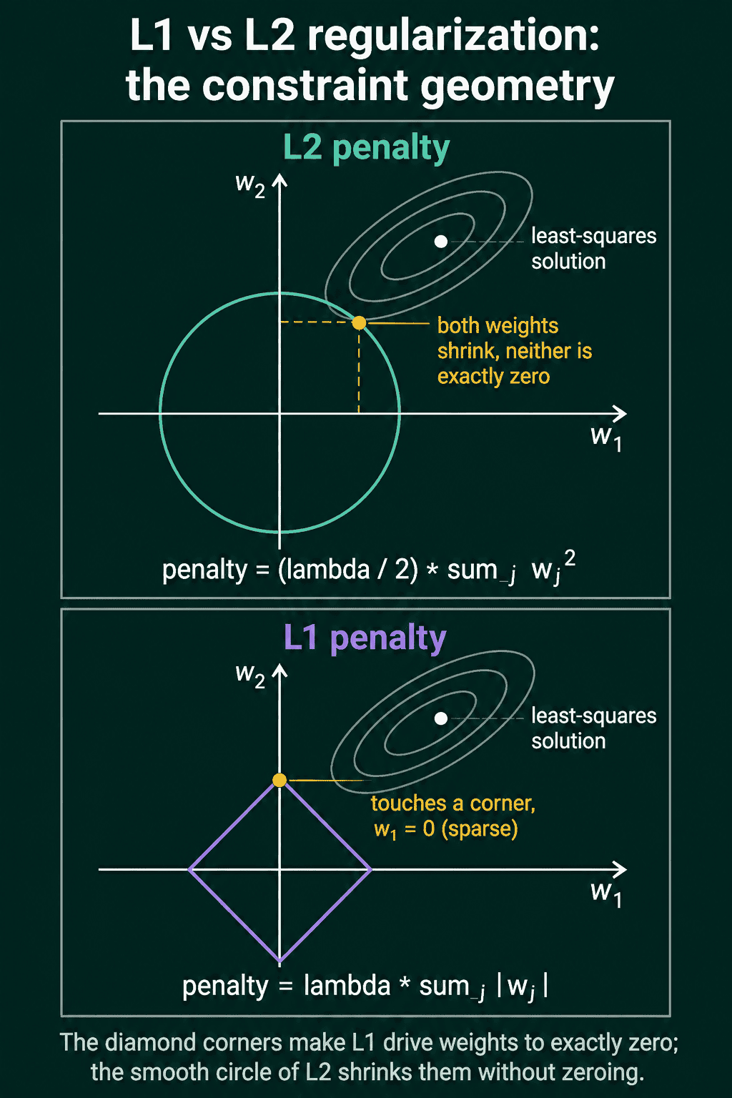
The picture shows the same fact geometrically for a model with two weights, $w_1$ and $w_2$. The ellipses are contours of the data loss, and the white dot in their center is the solution with no penalty. The penalty limits the weights to a region around zero: a circle for L2, a diamond for L1. The regularized solution is where the smallest ellipse touches the region. The circle is usually touched at a point where both weights are non-zero, and the diamond is usually touched at a corner, where one weight is exactly zero.
PyTorch optimizers have no L1 option, so you add the penalty to the loss yourself:
1l1_lambda = 1e-5
2l1_penalty = sum(p.abs().sum() for p in model.parameters())
3loss = criterion(model(x), y) + l1_lambda * l1_penalty
Dropout
Dropout works on neurons instead of weights. On each training step, it sets the output of a random fraction $p$ of the neurons in a layer to zero. With $p = 0.5$, half of the layer is switched off, and a different half is chosen at the next step.
Because any neuron might be missing on a given step, the neurons after it cannot depend on one specific neuron to carry a piece of information. The network tends to store each useful signal in several neurons, and features that survive this random removal are more likely to be useful beyond the exact training examples.
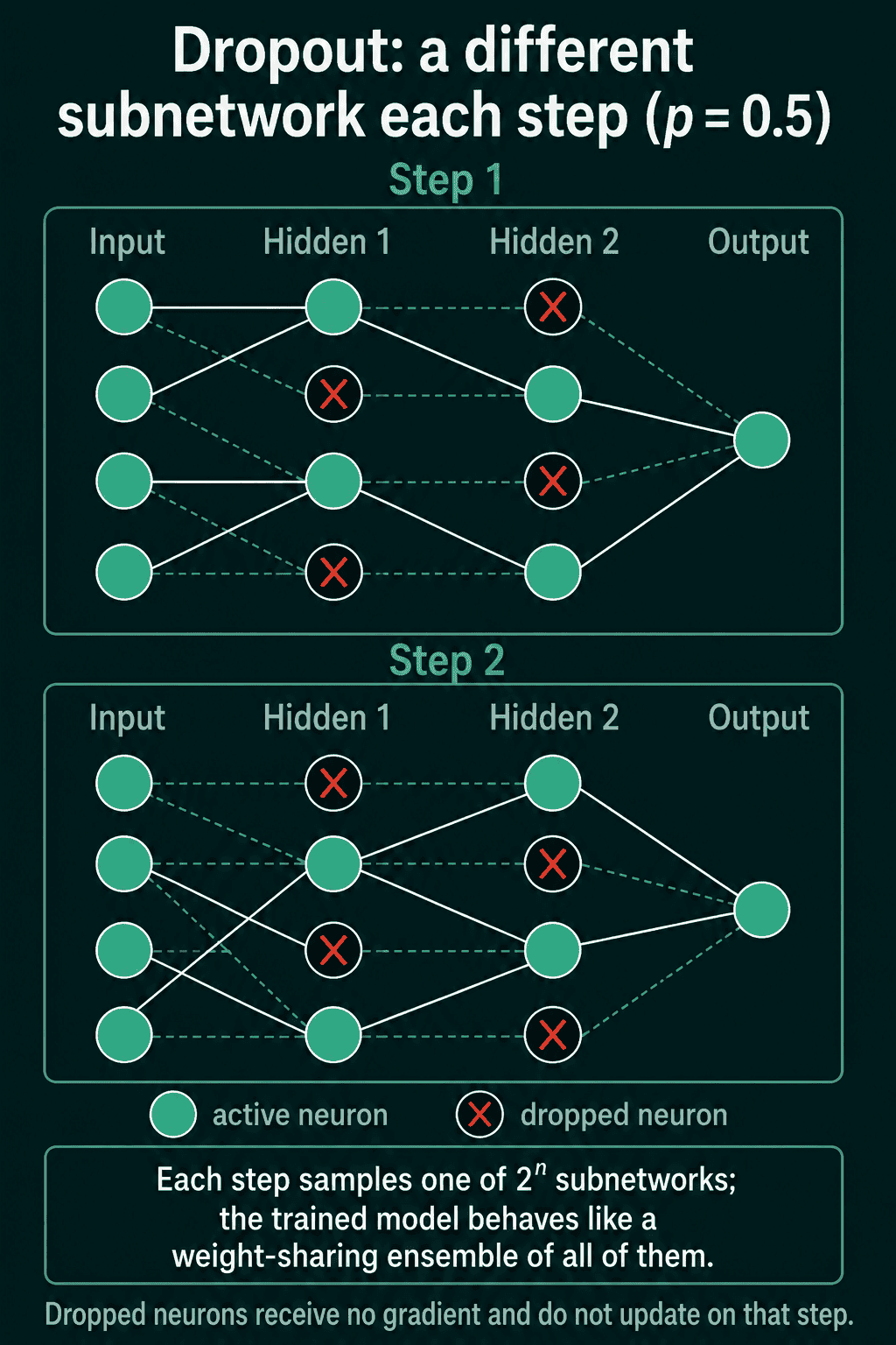
Each step trains a different subnetwork, meaning the network that remains after the dropped neurons are removed. A layer with $n$ neurons has $2^n$ possible subnetworks, and they all share the same weights. The trained model behaves somewhat like an ensemble, which is a group of models whose predictions are averaged.
At test time you want every neuron active. PyTorch handles this through the model's mode, and it rescales the surviving outputs during training by $\frac{1}{1-p}$ so the typical size of a layer's output is the same in both modes:
1import torch.nn as nn
2
3model = nn.Sequential(
4    nn.Linear(784, 256),
5    nn.ReLU(),
6    nn.Dropout(p=0.3),
7    nn.Linear(256, 10),
8)
9
10model.train()  # dropout active
11model.eval()   # dropout off, call this before validating or predicting
Values of $p$ between 0.1 and 0.5 are typical. Transformers often use 0.1, and fully connected layers in older architectures often use 0.5.
Early stopping
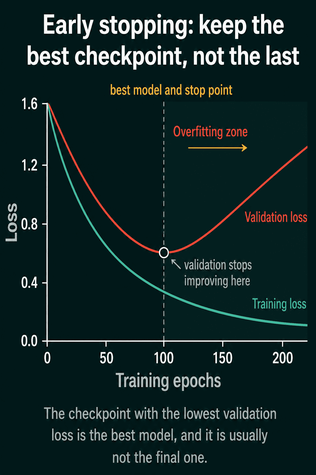
Early stopping limits how long the model trains. The more gradient steps a model takes, the more of the training set's specific details it can fit, including the noise. After each epoch (one pass over the training data) you measure validation loss, save the model whenever it improves, and stop once it has not improved for a set number of epochs. That number is called patience.
1best_val_loss = float("inf")
2patience, no_improve = 5, 0
3
4for epoch in range(max_epochs):
5    train_one_epoch(model, train_loader, optimizer)
6    val_loss = validate(model, val_loader)
7
8    if val_loss < best_val_loss:
9        best_val_loss = val_loss
10        no_improve = 0
11        torch.save(model.state_dict(), "best_model.pt")
12    else:
13        no_improve += 1
14        if no_improve >= patience:
15            break
16
17model.load_state_dict(torch.load("best_model.pt"))
The last line matters: the model you keep is the saved checkpoint with the lowest validation loss, which is usually an earlier one than the final epoch. If validation loss is noisy, raise patience to 10 or more before changing anything else.
Which one should you use?
| Technique | What it limits | Typical setting |
|---|---|---|
| L2 / weight decay | size of weights | weight_decay=0.01 |
| L1 | number of non-zero weights | l1_lambda=1e-5 |
| Dropout | reliance on single neurons | p=0.1 to p=0.5 |
| Early stopping | number of training steps | patience=5 to 10 |
These can be combined. A common starting point for neural networks is early stopping plus weight decay, with dropout added if the gap between training and validation loss is still large. More training data narrows the same gap and often helps more than any setting above, when you can get it.
Common mistakes
- Regularizing a model that is underfitting. If training loss is also high, the model is not memorizing anything, and regularization is likely to make it worse. Check that the model can fit the training data first.
- Forgetting
model.eval(). With dropout still active during validation, the validation numbers are usually worse and change from run to run. - Using
weight_decaywith Adam instead of AdamW. Intorch.optim.Adamthe decay is mixed into the gradient and gets rescaled per weight, so it behaves differently from the penalty above.AdamWapplies it directly to the weights. - Tuning regularization on the test set. Pick $\lambda$, $p$, and patience using the validation set, and touch the test set once at the end.
Related concepts
Overfitting and underfitting describe the two failures that regularization sits between, and the bias-variance tradeoff is the formal version: regularization accepts a small rise in bias (error from a model that is too limited) for a larger drop in variance (error from sensitivity to the particular training set). Data augmentation, label smoothing, and batch normalization also have regularizing effects, each through a different mechanism.
QuiddityML teaches weight decay, L1, dropout, and early stopping as separate concepts in the ML Foundation track, and the exercises include turning the weight decay equation into code, ordering the lines of the early stopping loop, and spotting the bug in a dropout implementation.