16 September 2026 · gradient-descentoptimizationml-foundationlearning-rate
What is a learning rate, and how do you pick one?
The learning rate is the number that most often decides whether a model trains well. This post explains what it does inside the update rule, how to read the three shapes of a loss curve, why good values differ between SGD and Adam, and a five-line test that finds a usable value.
The learning rate is a number that controls how far a model moves its parameters on each training step. It is usually written $\eta$ (eta) and set once when the optimizer is created. Many training problems that are not bugs in the code trace back to this one number, which is why it is worth understanding before adjusting other settings.
Where the learning rate sits
Training a model means repeating one update many times. The gradient $\nabla L(\theta)$ is the vector of partial derivatives of the loss $L$ with respect to the parameters $\theta$, and it points in the direction that increases the loss fastest. The update moves the opposite way, scaled by the learning rate:
$$ \theta \leftarrow \theta - \eta , \nabla L(\theta) $$
The gradient decides the direction. The learning rate decides the size of the step in that direction. A gradient of 2.0 with $\eta = 0.1$ moves the parameter by 0.2; the same gradient with $\eta = 0.001$ moves it by 0.002. Nothing else in the update changes, so the difference between a model that trains quickly and one that barely moves can come down to this one multiplier.
In PyTorch the number is the lr argument of the optimizer:
import torch

model = torch.nn.Linear(10, 1)
optimizer = torch.optim.SGD(model.parameters(), lr=0.01)
The three regimes
A loss curve is a plot of the loss value after each step. Its shape tells you which of three situations you are in.
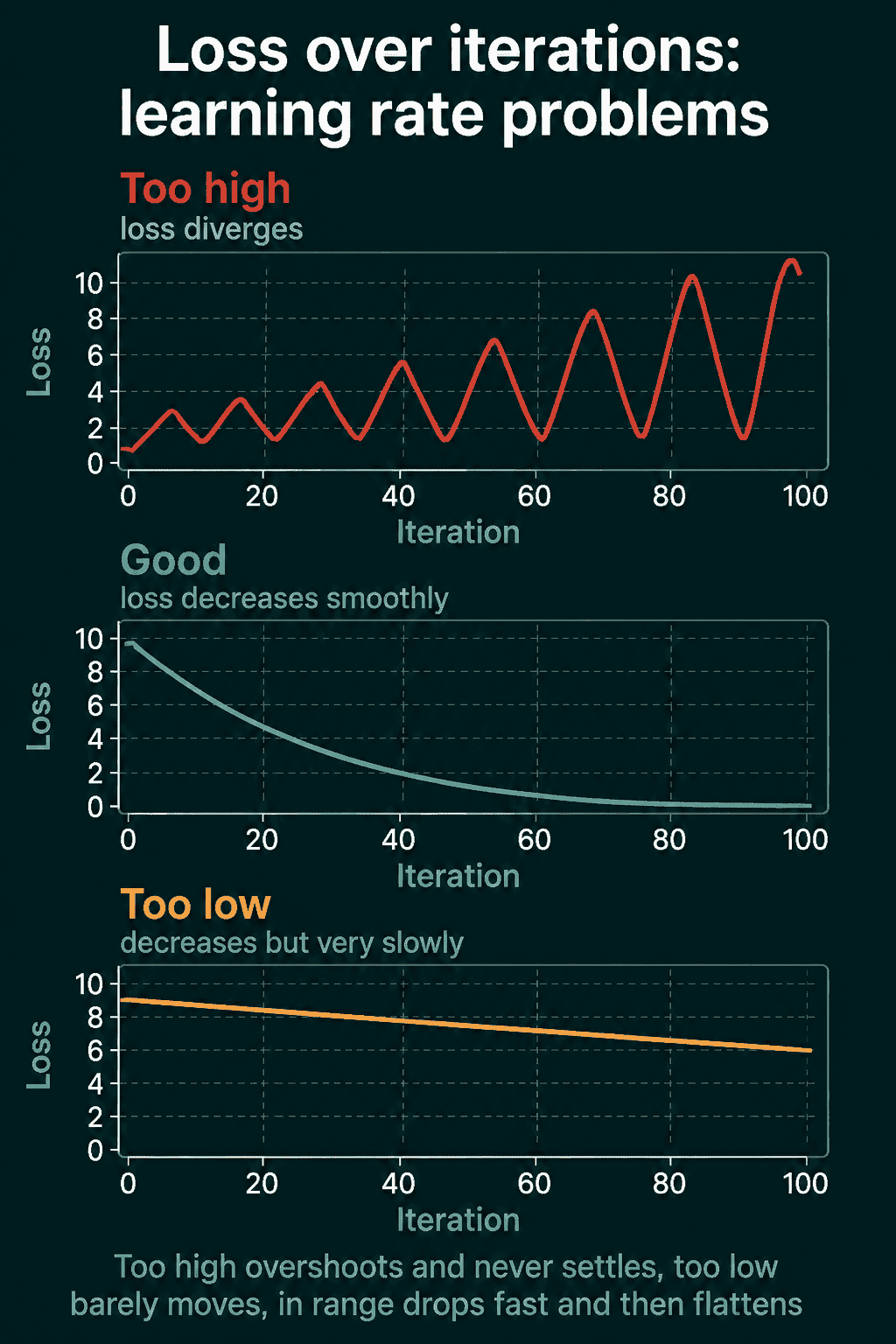
Too high. Each step overshoots the low point and lands on the far side, higher than before. The loss oscillates and grows, and often ends as nan once a value overflows. If the loss goes up on the first few steps or jumps around wildly, the learning rate is the first thing to lower.
Too low. Each step is so small that the loss barely changes. The curve slopes down but so slowly that a full run ends far from a good solution. This regime can be mistaken for a bug in the data or the model, because the loss does move, just not enough.
In range. The loss drops fast in the first steps and then flattens as the parameters approach a low point. Within the usable range, larger values reach the flat part sooner, so the goal is the largest value that still produces this smooth shape.
The usable range is wide, often a factor of 10 or more, so exact tuning is rarely needed. What is needed is to land inside it at all.
Why the right value does not transfer between setups
A learning rate that worked in one script is only a starting point in the next, because several other choices change what a given step size means.
- The optimizer. Plain SGD applies the raw gradient, so usable values are roughly 0.01 to 0.1. Adam divides each parameter's gradient by a running estimate of its size, which makes every step close to $\eta$ in magnitude regardless of the gradient. Its usable values are much smaller, typically 1e-4 to 3e-3, with 1e-3 as the common default.
- The batch size. The gradient is averaged over a batch. Larger batches give a less noisy gradient, which tolerates a larger step; a common rule is to scale the learning rate in proportion to the batch size when changing it.
- Normalization. Layers such as batch normalization keep activations at a stable scale, which makes the loss surface smoother and lets the model tolerate larger learning rates.
- The loss scale. Summing the loss over a batch instead of averaging multiplies the gradient by the batch size, which is the same as multiplying the learning rate by the batch size.
So the useful question is not "what is a good learning rate" but "what is a good learning rate for this optimizer, batch size, and model".
How to pick one
Start from the default for the optimizer. 1e-3 for Adam and AdamW, 0.01 for SGD without momentum, 0.1 for SGD with momentum on image models. These are inside the usable range for most small and medium problems.
Sweep by factors of 10. Train for a few hundred steps at 1e-4, 1e-3, 1e-2, and 1e-1 and compare the loss curves. Pick the largest value that still gives a smooth decrease, then optionally try 3 times larger and 3 times smaller. Because the usable range is wide, a coarse sweep is enough.
Run a learning rate range test. Start at a very small value and multiply it by a constant every step while recording the loss. The loss stays flat while the rate is too small, drops once it enters the usable range, and blows up once it is too large. A good choice is a value in the dropping section, somewhat below the point where the curve turns back up.
import math
import torch

model = torch.nn.Linear(10, 1)
optimizer = torch.optim.SGD(model.parameters(), lr=1e-6)
loss_fn = torch.nn.MSELoss()
X, y = torch.randn(256, 10), torch.randn(256, 1)

factor = math.exp(math.log(1e1 / 1e-6) / 100)  # 100 steps from 1e-6 to 10
for step in range(100):
    optimizer.zero_grad()
    loss = loss_fn(model(X), y)
    loss.backward()
    optimizer.step()
    print(f"lr={optimizer.param_groups[0]['lr']:.2e} loss={loss.item():.4f}")
    optimizer.param_groups[0]["lr"] *= factor
Every parameter group in the optimizer carries its own lr, which is why the code reads and writes param_groups[0]["lr"].
Changing it during training
A single constant value is a compromise: the value that makes fast progress early is often too large to settle precisely at the end. A learning rate schedule changes $\eta$ over the run.
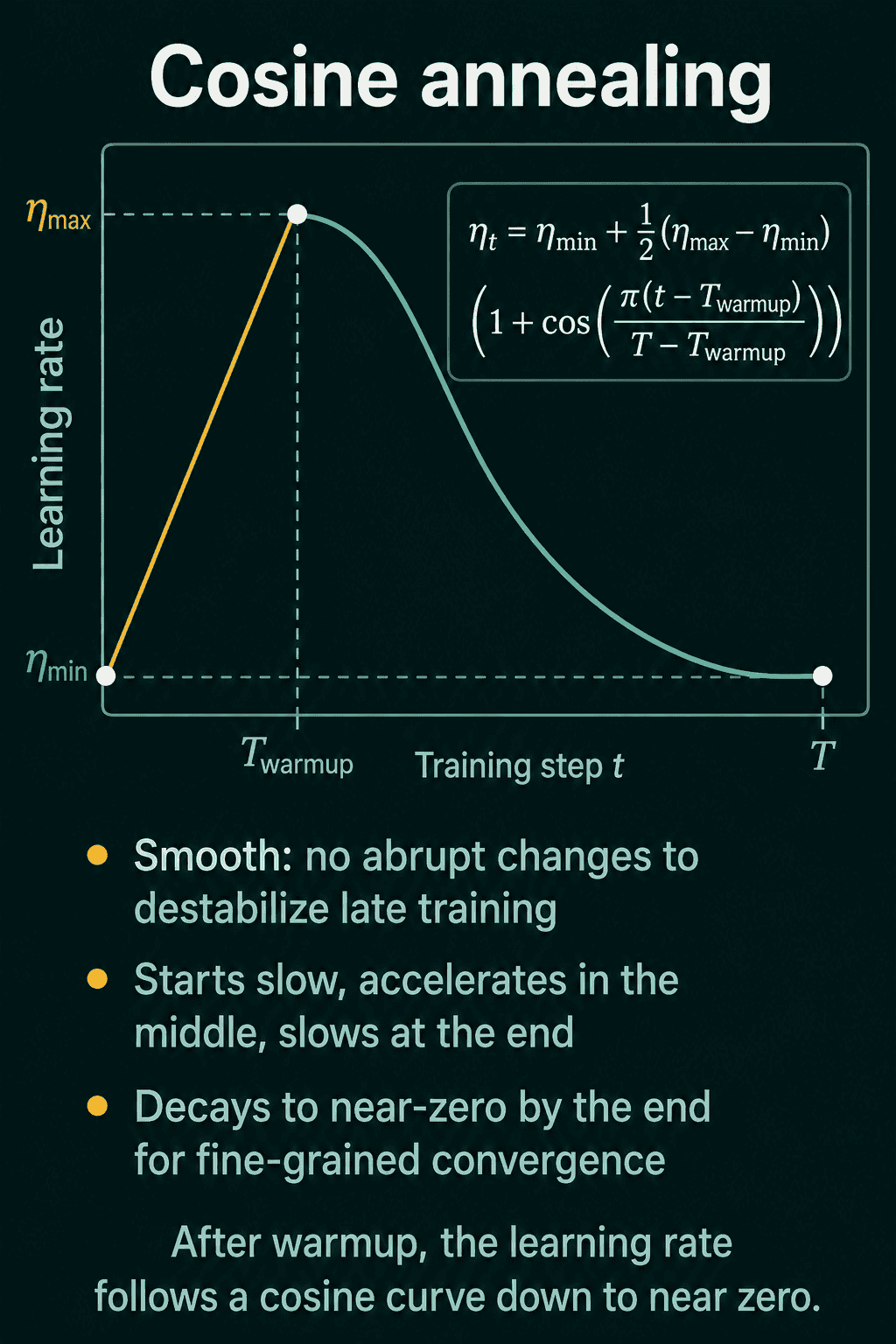
- Warmup ramps the rate linearly from near zero to the peak over the first few hundred steps. Adam's running estimates are unreliable at the start, and warmup stops the first steps from being too large.
- Step decay divides the rate by a fixed factor at chosen epochs, for example by 10 at epochs 30, 60, and 90.
- Cosine annealing decays the rate smoothly from the peak to near zero over the whole run, following half a cosine curve. It is a common choice for training transformers.
In PyTorch a scheduler wraps the optimizer and is stepped once per epoch or once per batch:
optimizer = torch.optim.AdamW(model.parameters(), lr=1e-3)
scheduler = torch.optim.lr_scheduler.CosineAnnealingLR(optimizer, T_max=1000)

for step in range(1000):
    optimizer.zero_grad()
    loss = loss_fn(model(X), y)
    loss.backward()
    optimizer.step()
    scheduler.step()
The scheduler step goes after the optimizer step; PyTorch warns if the order is reversed.
Common mistakes
- Using an SGD value with Adam.
lr=0.1with Adam takes a step of about 0.1 on every parameter on every update, which is far too large for most models. - Reading a flat loss as a model problem. Before changing the architecture, multiply the learning rate by 10 and look again.
- Tuning the learning rate before fixing the loss scale. Switching a loss from
sumtomeanchanges the gradient by the batch size and invalidates the previous value. - Forgetting the scheduler. Creating a scheduler without calling
scheduler.step()leaves the rate constant, silently. - Copying a value across batch sizes. Going from a batch of 32 to 256 without raising the rate makes training slower than it needs to be.
Related concepts
- Adam versus SGD: Adam normalizes step sizes per parameter, which is why its learning rates are smaller and why it is less sensitive to the exact value.
- Batch size: larger batches average out gradient noise and tolerate larger learning rates.
- Warmup: a short ramp at the start protects the first steps, when the optimizer's statistics are still empty.
- Gradient clipping: capping the gradient norm limits the damage of a single oversized step without lowering the rate for all steps.
QuiddityML teaches the learning rate as its own concept in the ML Foundation track, and its exercises include matching each of the three loss curves to its cause, spotting an Adam optimizer created with an SGD-sized learning rate, and predicting what a training loop prints when the scheduler step is missing.