21 September 2026 · backpropagationgradientsml-foundation

What is backpropagation? Explained with a tiny network

Backpropagation is how a neural network works out which way to change each of its weights to reduce its error. This post computes it by hand on a network with two weights, shows why it runs backward, and checks the numbers against PyTorch.

Backpropagation is the procedure a neural network uses to work out, for each of its weights, whether raising or lowering that weight would reduce the error, and by how much. Training a network means repeating two steps many times: measure the error, then nudge each weight in the direction that lowers it. Backpropagation supplies the directions for the second step, and loss.backward() in PyTorch is this procedure.

What problem does backpropagation solve?

A neural network turns an input into a prediction by passing it through layers, and each layer multiplies by weights, the adjustable numbers the network learns. The loss is a single number that says how wrong the prediction was. To improve, the network needs to know how the loss would change if one weight changed slightly. That quantity is the derivative of the loss with respect to the weight, and the collection of these derivatives for all weights is called the gradient.

The slow way to get it is to change one weight by a tiny amount, run the network again, and see how much the loss moved. That costs one full run of the network per weight. A model with 100 million weights would need 100 million runs for a single training step. Backpropagation gets all of the derivatives from one run forward and one run backward.

The chain rule on one small example

Backpropagation is the chain rule from calculus applied step by step. The chain rule says that when a value passes through several operations in a row, the derivative of the final result with respect to the starting value is the product of the derivatives of each operation.

Take $z = 3x^2 + 1$ at $x = 2$. Split it into three operations: square $x$ to get 4, multiply by 3 to get 12, add 1 to get 13. Each operation has its own derivative, called its local gradient. Squaring has local gradient $2x = 4$. Multiplying by 3 has local gradient 3. Adding 1 has local gradient 1.

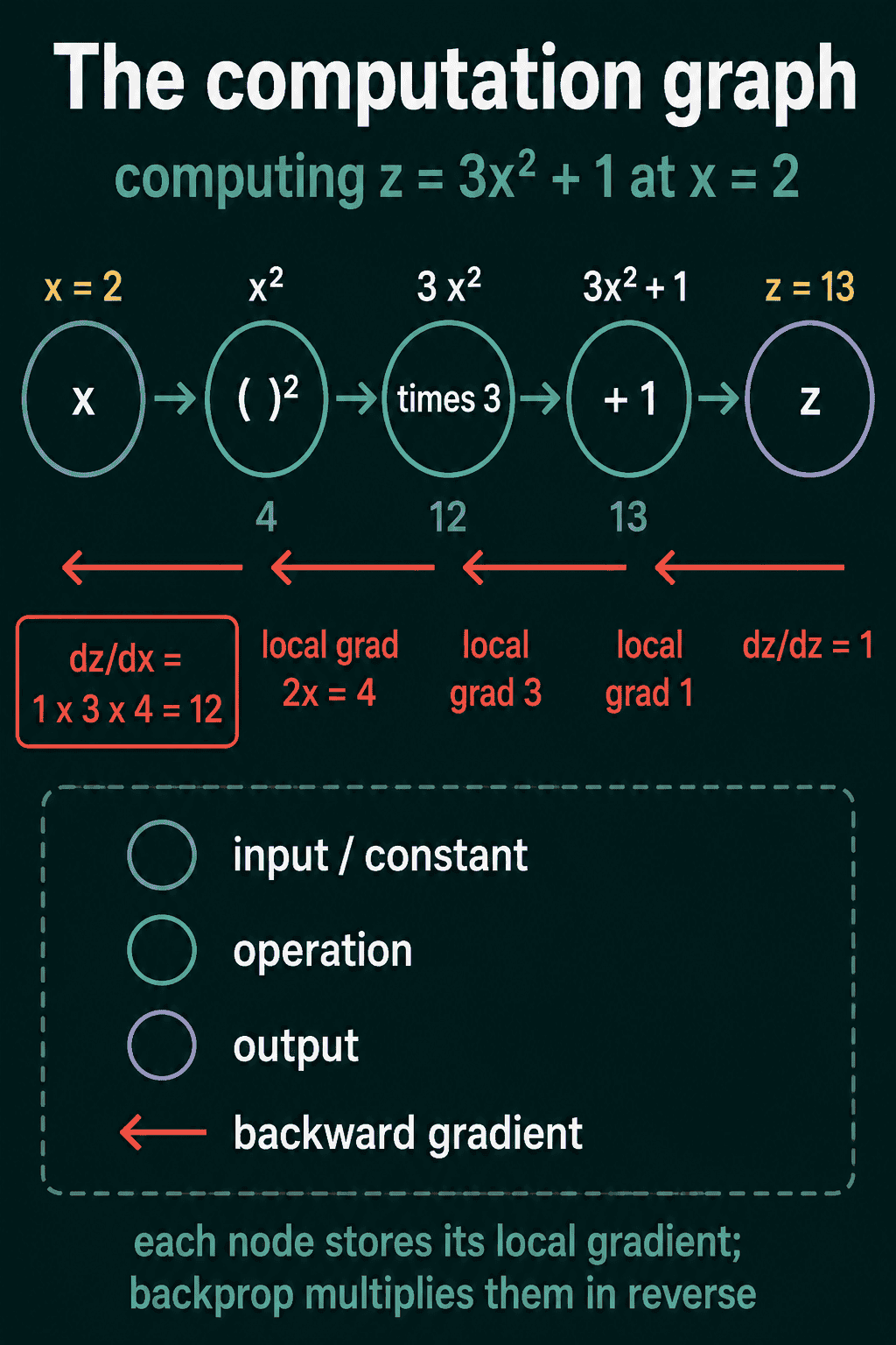
A chain of operations computing z = 3x squared + 1 at x = 2: square, times 3, plus 1, giving 13. Red arrows run backward from z to x, multiplying the local gradients 1, 3, and 4 to give dz/dx = 12.

Start at the output, where the derivative of $z$ with respect to itself is 1, and move backward, multiplying by each local gradient on the way: $1 \times 1 \times 3 \times 4 = 12$. That matches the derivative from calculus, $6x = 12$. This chain of operations is called a computation graph, and backpropagation is this backward walk over it.

A tiny network, computed by hand

Now the same thing on a network. It has one input $x$, one hidden neuron, and one output, with two weights $w_1$ and $w_2$. The hidden neuron uses ReLU, a function that keeps positive numbers and turns negative numbers into 0. The target value the network should output is $y$.

Set $x = 2$, $y = 1$, $w_1 = 0.5$, and $w_2 = 0.4$. Running the network from input to loss is called the forward pass:

$a = w_1 x = 0.5 \times 2 = 1.0$
$h = \text{ReLU}(a) = 1.0$
$\hat{y} = w_2 h = 0.4 \times 1.0 = 0.4$, the prediction
$L = (\hat{y} - y)^2 = (0.4 - 1)^2 = 0.36$, the loss

The backward pass starts at the loss and moves toward the input, one operation at a time.

The loss is a square, so its derivative with respect to the prediction is $2(\hat{y} - y)$:

$$\frac{\partial L}{\partial \hat{y}} = 2(0.4 - 1) = -1.2$$

The prediction is $w_2 h$. Its local gradient with respect to $w_2$ is $h$, and with respect to $h$ it is $w_2$:

$$\frac{\partial L}{\partial w_2} = -1.2 \times 1.0 = -1.2$$

$$\frac{\partial L}{\partial h} = -1.2 \times 0.4 = -0.48$$

ReLU has local gradient 1 when its input is positive and 0 otherwise. Here $a = 1.0$, so the gradient passes through unchanged, and $\frac{\partial L}{\partial a} = -0.48$. Finally $a = w_1 x$, whose local gradient with respect to $w_1$ is $x$:

$$\frac{\partial L}{\partial w_1} = -0.48 \times 2 = -0.96$$

Both gradients are negative, which means raising either weight lowers the loss. Gradient descent moves each weight against its gradient by a small multiple called the learning rate. With a learning rate of 0.1, $w_2$ becomes $0.4 + 0.12 = 0.52$ and $w_1$ becomes $0.5 + 0.096 = 0.596$. Run the forward pass again and the prediction is about 0.62, with a loss of about 0.145, down from 0.36.

Why does it run backward?

Look at how $\frac{\partial L}{\partial w_1}$ was computed. It reused $\frac{\partial L}{\partial h}$, which reused $\frac{\partial L}{\partial \hat{y}}$. Every weight in an early layer affects the loss only through the layers after it, so its gradient needs the gradients of those later layers. Starting from the loss and moving backward means each of those shared pieces is computed once and passed along, instead of being recomputed for every weight.

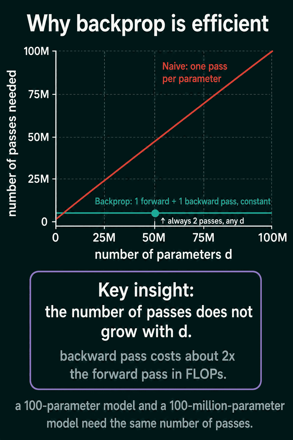
A plot of the number of network passes needed against the number of parameters. The naive method of one pass per parameter grows as a straight line to 100 million. Backpropagation stays flat at one forward and one backward pass.

This is why the cost does not grow with the number of weights in the way the slow method does. One training step is one forward pass and one backward pass, whatever the size of the model, and the backward pass costs roughly twice the arithmetic of the forward pass.

The same example in PyTorch

PyTorch records each operation during the forward pass, building the computation graph as it goes. Calling backward() on the loss walks that graph in reverse and stores each weight's gradient in its .grad attribute. This system is called autograd.

1import torch
2 
3x = torch.tensor(2.0)
4y = torch.tensor(1.0)
5w1 = torch.tensor(0.5, requires_grad=True)
6w2 = torch.tensor(0.4, requires_grad=True)
7 
8h = torch.relu(w1 * x)
9y_hat = w2 * h
10loss = (y_hat - y) ** 2
11 
12loss.backward()
13print(w1.grad, w2.grad)  # tensor(-0.9600) tensor(-1.2000)

The numbers match the hand calculation. In a real training loop the optimizer reads these .grad values and updates the weights, so most training code does not touch them directly. If a gradient prints as None, check first that the tensor was created with requires_grad=True and that it was used to compute the loss.

Common mistakes

Not clearing old gradients. PyTorch adds new gradients to whatever is already in .grad. Call optimizer.zero_grad() once per training step, or the gradients from earlier batches pile up.
Cutting the graph by accident. Calling .item(), .detach(), or converting to NumPy in the middle of the forward pass removes that value from the graph, so no gradient flows through it.
Dead ReLU neurons. If a ReLU neuron's input is negative for every example, its local gradient is 0 and the weights before it stop updating. In the example above, a starting $w_1$ of $-0.5$ would give $\frac{\partial L}{\partial w_1} = 0$.
Vanishing gradients. The backward pass multiplies local gradients together. Sigmoid has a local gradient of at most 0.25, so ten sigmoid layers in a row can shrink the gradient by a factor of about a million, and the early layers can learn very slowly. ReLU and normalization layers are common fixes.

Related concepts

Backpropagation computes the gradient and does nothing else. Gradient descent is the rule that uses the gradient to update the weights, and optimizers such as SGD and Adam are variations on that rule. Autograd is PyTorch's implementation of backpropagation for computations built from differentiable PyTorch operations, not only neural networks.

QuiddityML teaches backpropagation as its own concept in the ML Foundation track, moving from the chain rule to the computation graph to gradients for whole layers, with exercises that include picking the code that computes a layer's weight gradient and backpropagating by hand through a small computation graph.