16 September 2026 · gradient-descentoptimizationml-foundation

What is gradient descent? Explained step by step

Gradient descent is the procedure that trains almost every machine learning model. This post explains what it does, why the update has a minus sign, how the learning rate changes everything, and what the three lines of PyTorch that implement it are doing.

Gradient descent is a procedure that repeatedly nudges a model's parameters in the direction that makes its error smaller. It is how nearly every model you will meet gets trained, from a straight line fitted to ten points to a language model with billions of weights. If you understand this one loop, most of what an "optimizer" does in a training script stops being magic.

What problem does it solve?

A model is a function with adjustable numbers inside it, called parameters or weights and biases. A loss function is a second function that takes the model's predictions and the true answers and returns one number: how wrong the model is right now. Training means finding the parameter values that make that number as small as possible.

You cannot try every combination. A small network has millions of parameters, each a real number, so there is no list to search through. What you can do is ask, for the current parameters, which direction would make the loss go down, and move a little that way. Then ask again. Gradient descent is that question asked over and over.

The simplest version: one parameter

Imagine a model with a single weight $w$, and plot the loss $L$ against every value of $w$. For many problems the plot is a bowl: high on both sides, lowest somewhere in the middle. You are standing on the side of the bowl at your current $w$ and want to reach the bottom.

The slope of the curve at your position tells you everything you need. If the slope is positive, the loss increases as $w$ increases, so you should decrease $w$. If the slope is negative, you should increase $w$. Either way, move against the slope. The slope of a function at a point is its derivative, so the rule is: take a step in the direction opposite to the derivative, then measure the slope again from the new spot.

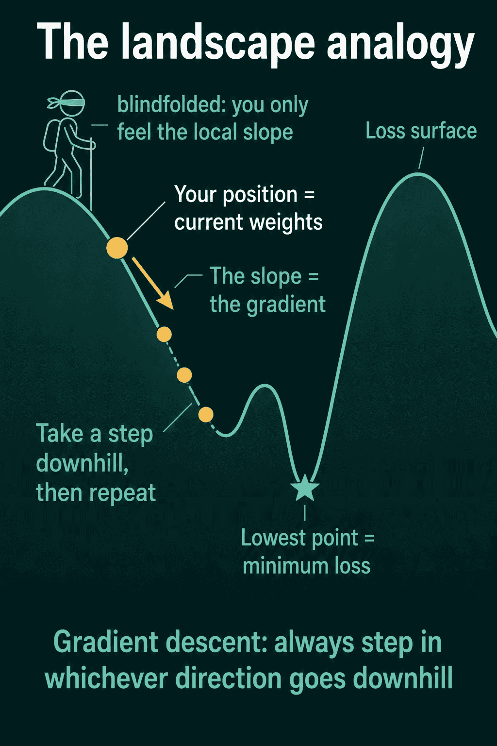
A curved loss surface with a dot stepping downhill along the slope toward the lowest point, with the slope labeled as the gradient

That is the entire idea. Everything else in this post is the same move with more than one parameter, and the details of how big a step to take.

The real mechanism: the gradient

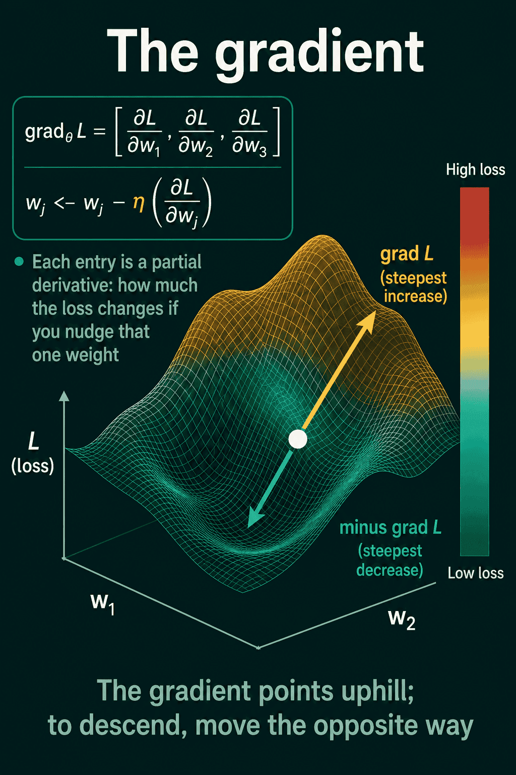
With many parameters, the loss depends on all of them at once. The derivative of the loss with respect to one parameter, holding the others fixed, is called a partial derivative. It answers: if I nudge this one weight up a little, how much does the loss change?

The gradient is the list of all those partial derivatives, one per parameter, written as a vector. It is written $\nabla L$ (read "grad L"). The gradient has a useful property: as a direction in parameter space, it points the way the loss increases fastest. So the direction that decreases the loss fastest is the exact opposite, $-\nabla L$.

The update rule

Call the full set of parameters $\theta$ and the learning rate $\eta$, a small positive number you choose that controls how big each step is. One step of gradient descent is:

$$ \theta \leftarrow \theta - \eta , \nabla L(\theta) $$

In words: compute the gradient of the loss at the current parameters, scale it by the learning rate, and subtract it from the parameters. The minus sign is what makes this descent rather than ascent. For a single weight $w_j$ the same rule reads $w_j \leftarrow w_j - \eta , \partial L / \partial w_j$, which is the picture below.

The gradient as a vector of partial derivatives, the update rule for one weight, and a 3D loss surface with an arrow pointing uphill along the gradient and another pointing downhill along its negative

Training repeats this update thousands or millions of times. Each repetition is one step; a pass over the whole dataset is an epoch.

Why the learning rate decides everything

The learning rate $\eta$ is the one number in this rule you have to pick, and both directions of being wrong are visible in the loss curve.

Too small, and each step barely moves. The loss goes down, but so slowly that training takes far longer than it should, and it may stop before reaching anything good.

Too large, and a step can jump right over the bottom of the bowl to the other side, where the slope is now steeper, so the next step jumps even further. The loss goes up instead of down, oscillates, or becomes infinite and prints as NaN.

A common starting choice is $0.01$ for plain gradient descent and $0.001$ for Adam, then adjusting by factors of 10 based on the loss curve. If the loss explodes, divide the learning rate by 10. If it crawls, multiply by 10.

The code

Here is gradient descent for a straight line $y = wx + b$ fitted to a few points, with the update written out by hand so nothing is hidden:

import torch

x = torch.tensor([1.0, 2.0, 3.0, 4.0])
y = torch.tensor([3.0, 5.0, 7.0, 9.0])   # the true line is y = 2x + 1

w = torch.zeros(1, requires_grad=True)
b = torch.zeros(1, requires_grad=True)
lr = 0.01

for step in range(2000):
    pred = w * x + b
    loss = ((pred - y) ** 2).mean()   # mean squared error
    loss.backward()                    # fills w.grad and b.grad with the gradient
    with torch.no_grad():
        w -= lr * w.grad               # the update rule, one line per parameter
        b -= lr * b.grad
        w.grad.zero_()                 # gradients accumulate, so clear them
        b.grad.zero_()

print(w.item(), b.item())              # close to 2.0 and 1.0

The call to backward() computes every partial derivative for you, and the two lines inside no_grad are the update rule. In real code the same thing is written with an optimizer object, which does exactly those lines:

opt = torch.optim.SGD([w, b], lr=0.01)
for step in range(2000):
    opt.zero_grad()
    loss = ((w * x + b - y) ** 2).mean()
    loss.backward()
    opt.step()

If this diverges, the first thing to change is the learning rate.

When it works, and the mistakes people make

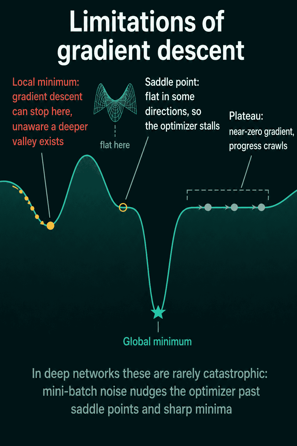
Gradient descent finds a point where the gradient is zero, which is a minimum of the loss if the surface is bowl-shaped there. On a plain bowl it will reach the bottom given enough steps and a sensible learning rate. On more complex surfaces it can settle into a local minimum (a dip that is not the lowest one), stall on a saddle point (flat in some directions), or crawl across a plateau where the gradient is tiny. In deep networks these turn out to matter less than the picture suggests, mostly because of the noise introduced by training on small random batches, covered below.

The two mistakes that actually bite:

Forgetting to zero the gradients. PyTorch adds each new gradient onto the old one. Without zero_grad() every step uses the sum of all previous gradients, and the model flies off.
The learning rate. Nearly every "my loss is not decreasing" and "my loss is NaN" is this number. Change it before changing anything else.

QuiddityML teaches gradient descent as its own concept in the ML Foundation track, and the exercises on it include writing the update rule from the equation, spotting the missing zero_grad() in a training loop, and ordering the lines of the loop above from memory.

Related: SGD, mini-batches, momentum, Adam

The rule above computes the gradient on the whole dataset each step, which is called batch gradient descent and is too slow for real data. Stochastic gradient descent (SGD) computes the gradient on one example at a time, and mini-batch gradient descent, the version everyone actually uses, on a small random batch of 32 to 512 examples. Each step is cheaper and slightly noisy, and that noise is what lets training escape saddle points and shallow dips.

Three failure spots on a loss curve: a local minimum, a saddle point, and a plateau, with a note that mini-batch noise usually pushes past them

Momentum keeps a running average of past gradients and steps along that average, which smooths the noise and speeds up progress along consistent directions. Adam adds a second running average of squared gradients and divides by its square root, so each parameter gets its own effective step size; it is the default optimizer for most deep learning today. Both are gradient descent with a smarter choice of step, and the update rule above is the thing they are modifying.