By Sagi Shaier · 30 October 2026 · 8 min read

Bag of words, co-occurrence matrices, and PMI: count-based word vectors

How counting the words around each word turns raw text into vectors, with PyTorch code for a bag-of-words vector, a co-occurrence matrix and PPMI, and what each of them loses.

Count-based word vectors describe each word by tallies of the words that appear near it in a large pile of text. No training and no gradients are involved, so the numbers in the vector are counts, sometimes reweighted. They are cheap to build and make a solid baseline. The learned embeddings used in modern models chase the same statistics, so count-based vectors are a good way to see what a word vector holds.

Where the numbers have to come from

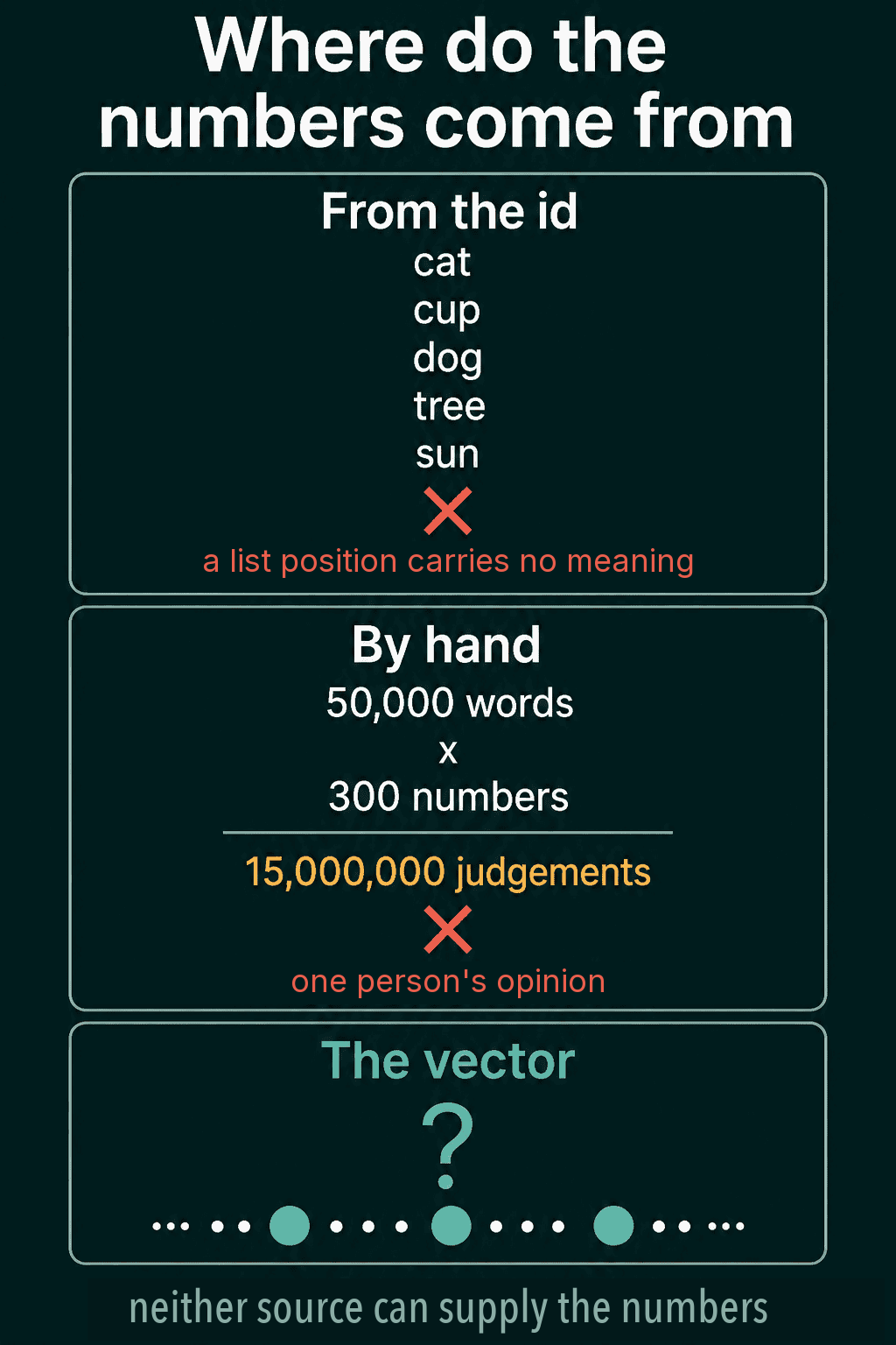
A model works best when each word gets a short list of numbers, called a dense vector, arranged so related words get similar numbers. Those numbers cannot come from the word's id or from a one-hot vector, because neither ever looks at text. An id records where a word landed in the tokenizer's list, and a vocabulary list records which words exist without saying anything about what they mean.

Writing the numbers by hand does not scale either. Three hundred numbers for each of 50,000 words is 15 million judgements, and they would be one person's opinion rather than anything measurable.

Two sources ruled out for a word's numbers: the id, which carries a list position and no meaning, and filling 15,000,000 numbers by hand

The distributional hypothesis

What a pile of raw sentences offers is the neighbours of every word. Cat and dog both turn up near pet, vet, food and play. Coffee and tea both turn up near cup, morning and drink. Read enough sentences that contain an unfamiliar word and you can work out roughly what it means without anyone defining it.

The distributional hypothesis states this: words that appear in similar contexts tend to mean similar things. The phrase usually quoted for it is "you shall know a word by the company it keeps."

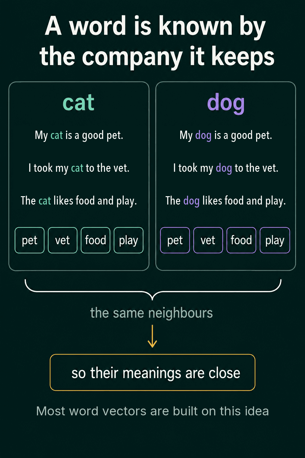
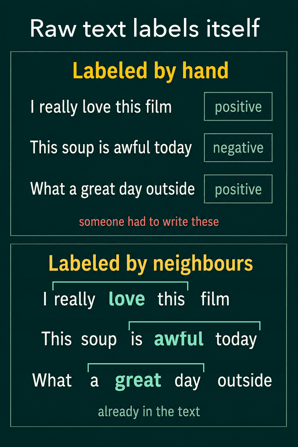
Three sentences each for cat and dog sharing the same neighbours pet, vet, food and play, so their meanings are close

The idea turns a hard question about meaning into a question about which words appear near which, and that is counting. It also scales well, because raw text needs no annotation. Each word's neighbours are already sitting next to it, so even a rare word can be placed from a handful of unlabelled sentences.

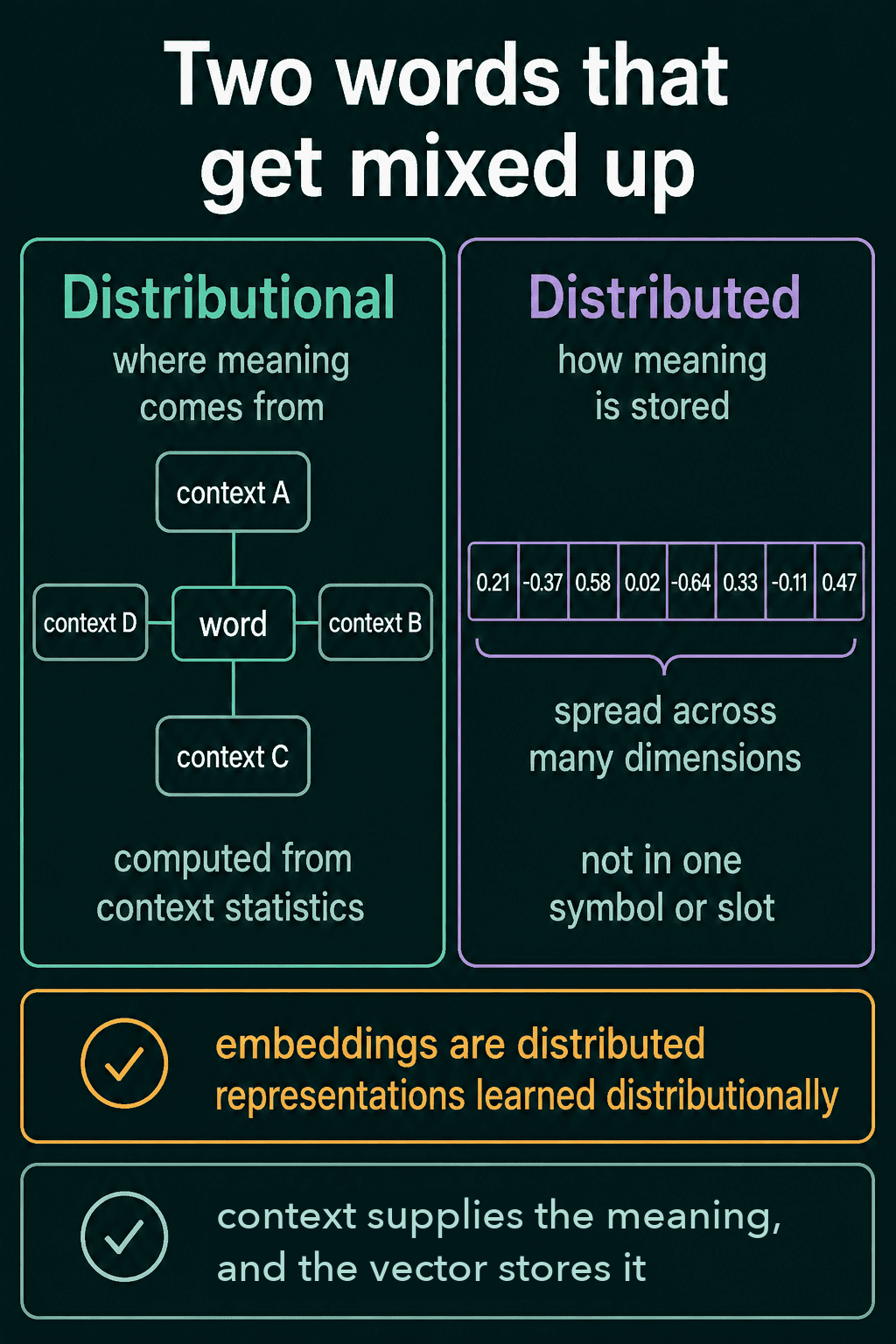
Sentences labelled positive or negative by hand compared with the same sentences where each word's neighbours are already in the text

Two similar-sounding terms come up here. Distributional is about where meaning comes from: it is computed from context statistics. Distributed is about how meaning is stored: it is spread across many dimensions of a vector rather than sitting in one. Most word embeddings are distributed representations estimated from distributional statistics.

Distributional means meaning comes from context statistics, and distributed means meaning is spread across many dimensions of a vector

Counting the company a word keeps

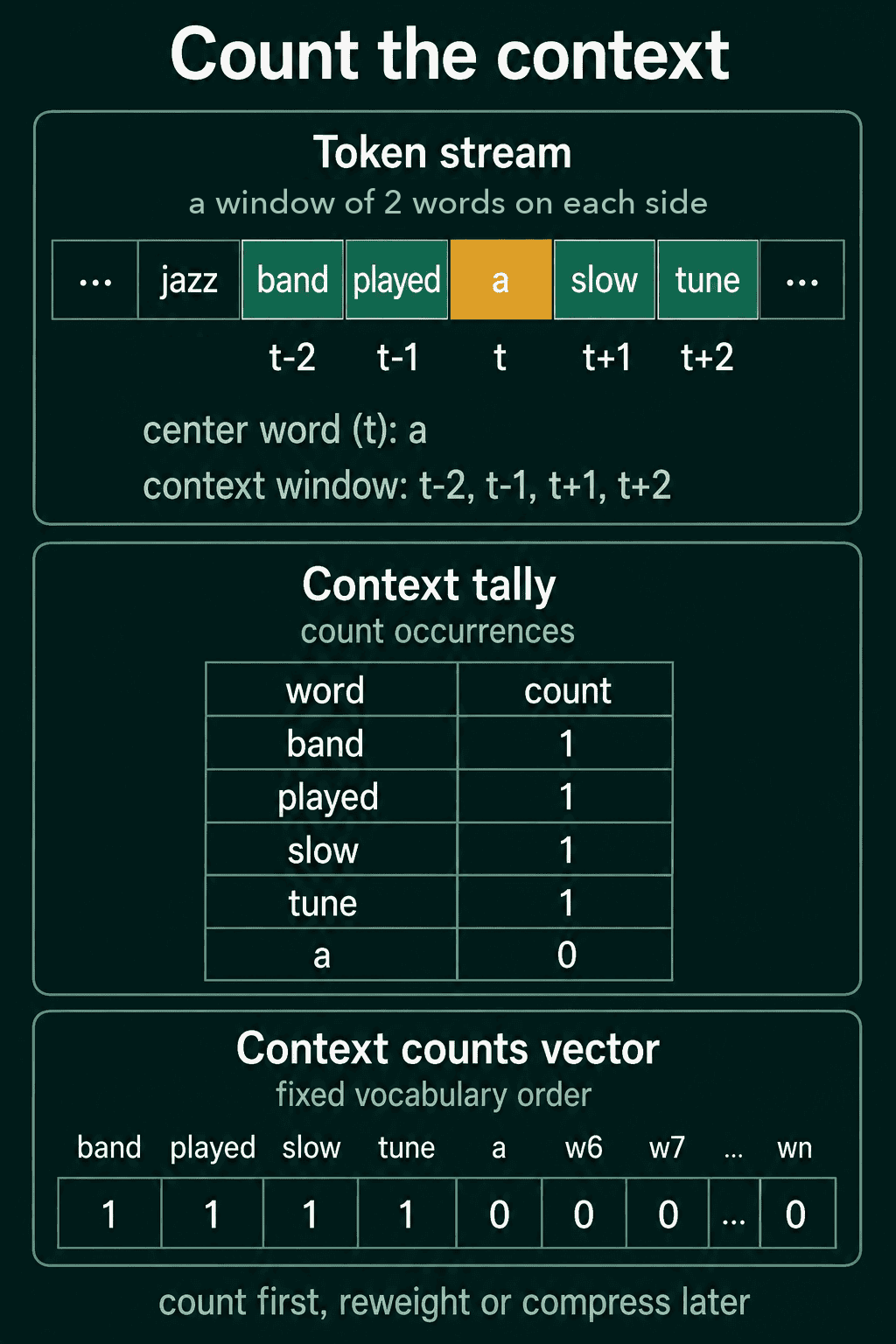
A count-based method walks through the text, tallies what appears next to what, and turns the tallies into vectors. The word whose company is being counted is the target word, and the words counted around it are its context.

A window of 2 words on each side of the word a, with band, played, slow and tune each counted once

Context window size

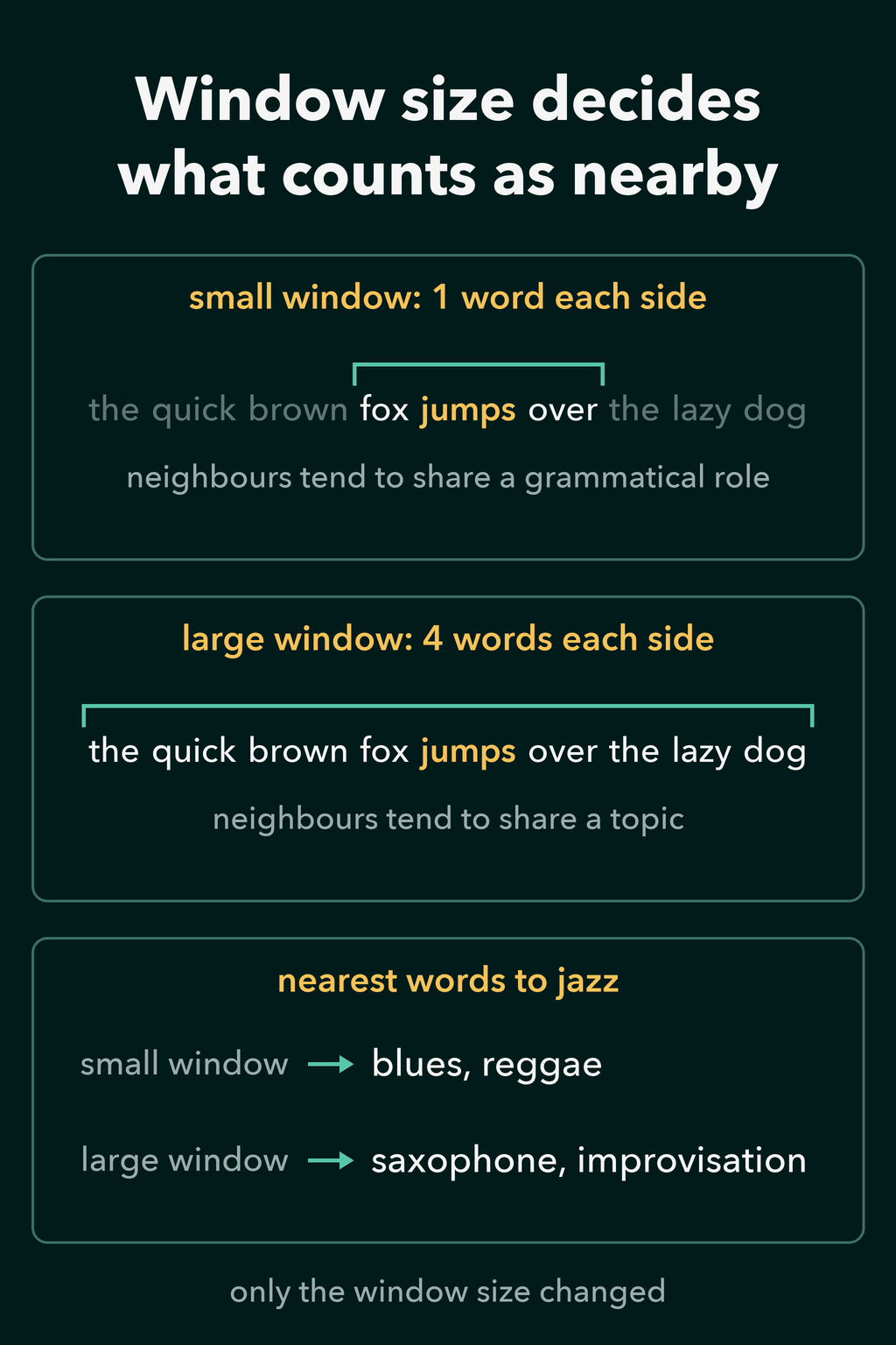
The context window is how many words on each side count as nearby. It is a setting you choose, and it changes what kind of similarity the vectors pick up.

With a narrow window of a word or two on each side, the closest matches to a word tend to share its grammatical role, so nouns match nouns and verbs match verbs. With a wide window of ten words or more, the matches share a topic whatever their part of speech. In one corpus, a narrow window puts jazz near other genre names such as blues and reggae, while a wide window puts it near saxophone and improvisation.

A one-word window around jumps covers fox and over, a four-word window covers the whole sentence, and for jazz the small window finds blues and reggae while the large one finds saxophone and improvisation

Bag of words

The simplest count-based representation describes a whole document instead of a single word. Bag of words represents a document as a vector with one dimension per vocabulary word, where dimension $i$ holds how many times word $i$ appears in that document.

1import torch
2 
3vocab = {'i': 0, 'liked': 1, 'the': 2, 'film': 3, 'hated': 4}
4 
5def bag_of_words(doc, vocab):
6    vec = torch.zeros(len(vocab))
7    for word in doc:
8        if word in vocab:
9            vec[vocab[word]] += 1
10    return vec
11 
12print(bag_of_words(['i', 'liked', 'the', 'film'], vocab))
13# tensor([1., 1., 1., 1., 0.])
14print(bag_of_words(['the', 'film', 'i', 'liked'], vocab))
15# tensor([1., 1., 1., 1., 0.])
16print(bag_of_words(['i', 'hated', 'the', 'film'], vocab))
17# tensor([1., 0., 1., 1., 1.])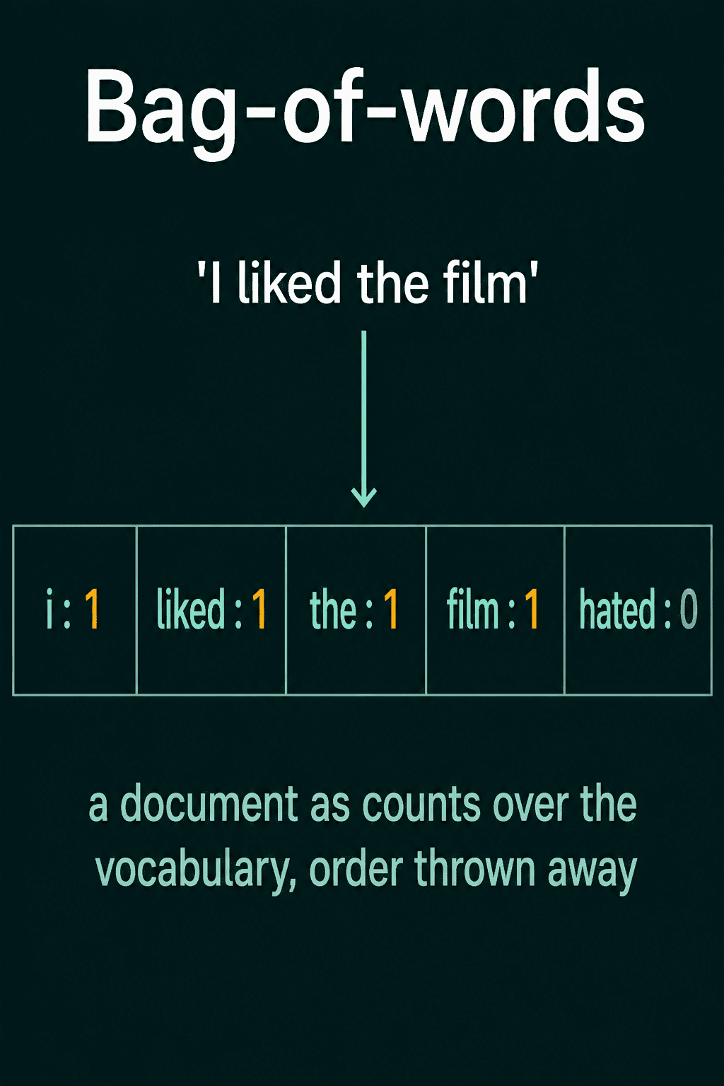

The document I liked the film turned into counts i 1, liked 1, the 1, film 1, hated 0

Two documents become two count vectors of the same length, and cosine similarity compares them directly. Cosine similarity is the dot product of two vectors divided by both their lengths, so it is 1 for vectors pointing the same way and 0 for vectors with nothing in common.

The name is literal: the words go into a bag and their positions are forgotten. The second call above shows it, since a shuffled sentence gives the same vector. Help, not harm and harm, not help also produce identical vectors although the order flips the meaning.

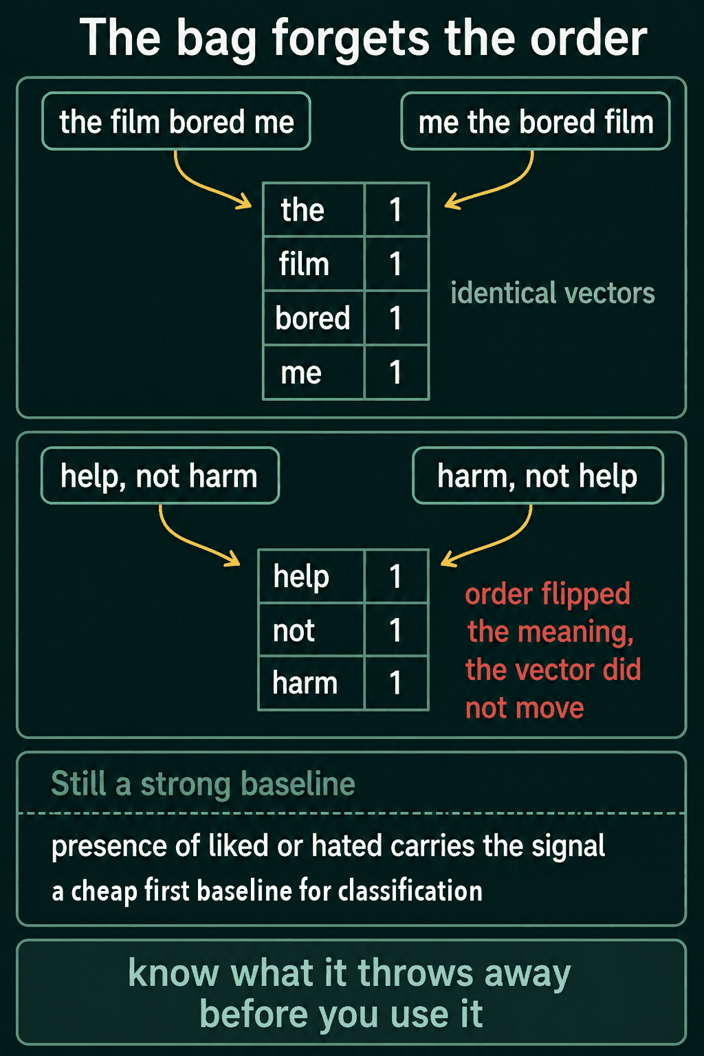
The film bored me and me the bored film give the same count vector, and so do help, not harm and harm, not help

Even so, bag of words is a cheap first baseline for classification. When sorting reviews into positive and negative, the presence of liked or hated carries most of the signal, and word order often carries less of it than you would expect.

Co-occurrence matrices

Bag of words counts words against documents. To get a vector for each word, count words against other words. A co-occurrence matrix $M$ has one row and one column per vocabulary word, and entry $M_{ij}$ is the number of times word $j$ appeared inside the window around word $i$.

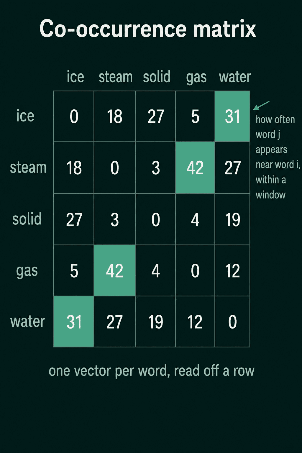
A co-occurrence matrix for ice, steam, solid, gas and water, where each cell counts how often one word appears near another

Each row is a word vector: the row for coffee is a tally of the company coffee keeps. Here is a small corpus with a window of 2 words on each side. The periods count as tokens too, and windows run across sentence ends.

1import torch
2import torch.nn.functional as F
3 
4text = ("i drink coffee every morning . i drink tea every morning . "
5        "a hot cup of coffee . a hot cup of tea . "
6        "i bake bread in the oven . fresh bread from the oven .")
7tokens = text.split()
8vocab = {w: i for i, w in enumerate(dict.fromkeys(tokens))}
9 
10def cooccurrence(tokens, vocab, window):
11    n = len(vocab)
12    M = torch.zeros(n, n)
13    for i, w in enumerate(tokens):
14        start = max(0, i - window)
15        end = min(len(tokens), i + window + 1)
16        for j in range(start, end):
17            if i != j:
18                M[vocab[w], vocab[tokens[j]]] += 1
19    return M
20 
21M = cooccurrence(tokens, vocab, window=2)
22 
23def neighbours(word):
24    row = M[vocab[word]]
25    return {w: int(row[i]) for w, i in vocab.items() if row[i] > 0}
26 
27print(neighbours('coffee'))
28# {'i': 1, 'drink': 1, 'every': 1, 'morning': 1, '.': 1, 'a': 1, 'cup': 1, 'of': 1}
29print(neighbours('tea'))
30# {'i': 2, 'drink': 1, 'every': 1, 'morning': 1, '.': 1, 'cup': 1, 'of': 1}
31print(M[vocab['coffee'], vocab['tea']].item())
32# 0.0
33 
34def similarity(a, b):
35    return F.cosine_similarity(M[vocab[a]], M[vocab[b]], dim=0).item()
36 
37print(round(similarity('coffee', 'tea'), 3))     # 0.894
38print(round(similarity('coffee', 'bread'), 3))   # 0.224

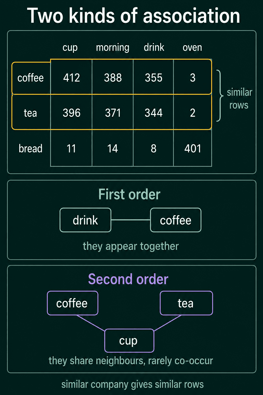
Coffee and tea never appear within two words of each other, since their cell is 0, and their rows still score 0.894 because they keep the same company. Coffee and bread share fewer neighbours and score 0.224.

That shows two kinds of association. First-order association links words that appear together, like drink and coffee. Second-order association links words that share neighbours, like coffee and tea. Comparing rows measures second-order association.

Coffee and tea have similar rows of counts for cup, morning, drink and oven, while bread's row is different, with drink and coffee as a first-order pair and coffee and tea linked through cup as a second-order pair

Counting words against documents instead of against neighbouring words gives a related table, the term-document matrix, where a word is described by which documents it appears in.

PMI and PPMI

Raw counts favour common words. A word like the sits next to most of the vocabulary, so it piles up large counts with almost every word without saying anything specific about any of them.

Pointwise mutual information (PMI) asks a different question: do two words appear together more often than chance would predict? Write $P(a, b)$ for the probability that words $a$ and $b$ appear together in a window, and $P(a)$ and $P(b)$ for how often each word appears on its own:

$$\text{PMI}(a, b) = \log_2 \frac{P(a, b)}{P(a)\,P(b)}$$

The bottom of the fraction is how often the pair would appear together if the two words had nothing to do with each other. For example, if $a$ appears in 10% of positions and $b$ in 2%, independent words would meet with probability $0.1 \times 0.02 = 0.002$. If they actually meet with probability $0.008$, the ratio is 4 and PMI is $\log_2 4 = 2$. Meeting exactly as often as chance gives PMI 0, and meeting more often gives a positive PMI.

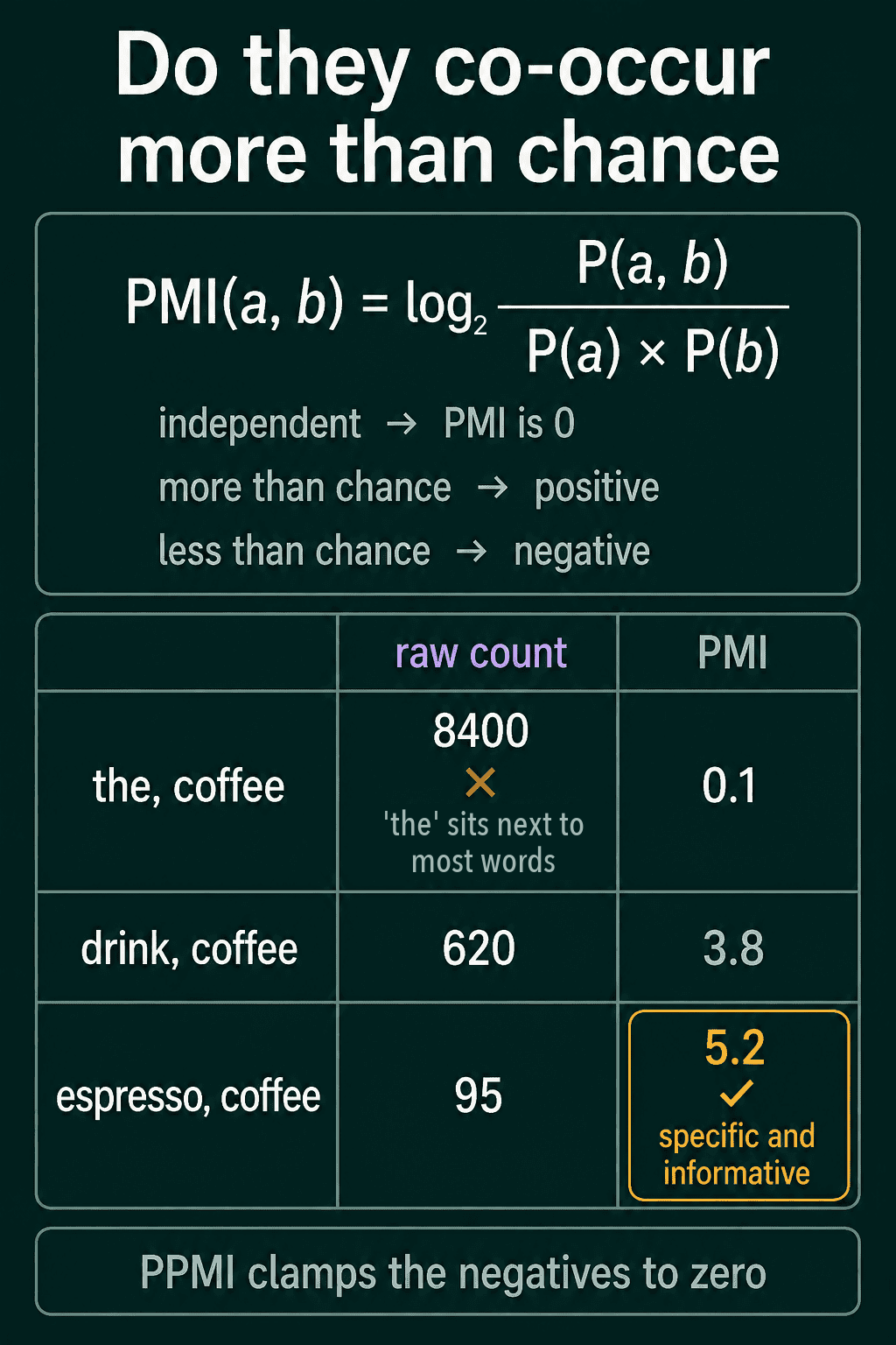
PMI compares how often two words appear together with chance: the and coffee have a raw count of 8,400 but PMI 0.1, while espresso and coffee have a raw count of 95 and PMI 5.2

A negative PMI would mean two words meet less often than chance predicts. Most pairs are expected to meet less than once in the whole corpus, so seeing them together zero times says little. Positive PMI (PPMI) sets every negative value to 0 and keeps only the pairs that meet more often than chance.

Continuing from the code above, PPMI turns the count matrix into probabilities and applies the formula to every cell:

1def ppmi(M):
2    total = M.sum()
3    p_ab = M / total
4    p_a = M.sum(dim=1, keepdim=True) / total
5    p_b = M.sum(dim=0, keepdim=True) / total
6    pmi = torch.log2(p_ab / (p_a * p_b))
7    return pmi.clamp(min=0)   # log2(0) is -inf, clamp turns it into 0
8 
9P = ppmi(M)
10for w in ['drink', 'cup', '.']:
11    print(w, int(M[vocab['coffee'], vocab[w]]), round(P[vocab['coffee'], vocab[w]].item(), 2))
12# drink 1 1.34
13# cup 1 1.15
14# . 1 0.0

Coffee appears once each next to drink and cup and the period, so the raw counts rank them equally. The period sits next to almost everything in the corpus, which brings its PPMI with coffee down to 0, while drink and cup keep positive scores.

When to use count-based vectors, and common mistakes

Use bag of words as a first baseline for document classification, such as sorting reviews into positive and negative. Move to something else when word order changes the label.
Pick the context window for the similarity you want. A narrow window groups words by grammatical role and a wide one groups them by topic.
Reweight before comparing rows. Raw counts let frequent words like the dominate every row, and PPMI removes much of that effect.
Expect long, sparse vectors. A co-occurrence row has one dimension per vocabulary word, so a 50,000-word vocabulary gives 50,000-dimensional rows that are mostly zeros. Count vectors usually need a separate compression step before they become short dense vectors.

The rows built here are word vectors made by counting. The post on turning words into numbers covers the measures used to compare them, including cosine similarity, and why ids and one-hot vectors cannot show which words are related. The post on word embeddings covers vectors learned from data instead of counted, which come out short and dense from the start.

QuiddityML teaches count-based vectors in the word representations unit of its NLP track, and the exercises include writing the co-occurrence function from scratch and spotting the loop that counts each word as its own neighbour (QuiddityML).