By Sagi Shaier · 7 October 2026 · 6 min read

Exponents and logarithms for machine learning

Logarithms show up in most machine learning loss functions because a log turns a product into a sum. This post covers the exponent and log rules, what an inverse function is, and why training works with log-likelihood instead of multiplying probabilities, with PyTorch code.

A logarithm is the power you have to raise a base to in order to get a number, so $\log_2(8) = 3$ because $2^3 = 8$. In machine learning, logs show up in most loss functions and likelihoods for one reason: a log turns a product into a sum. Sums are easier to differentiate, and they avoid a numerical failure where multiplying many small probabilities rounds to zero.

Logs and exponents undo each other, so this post starts with what it means for one function to undo another.

What a function is

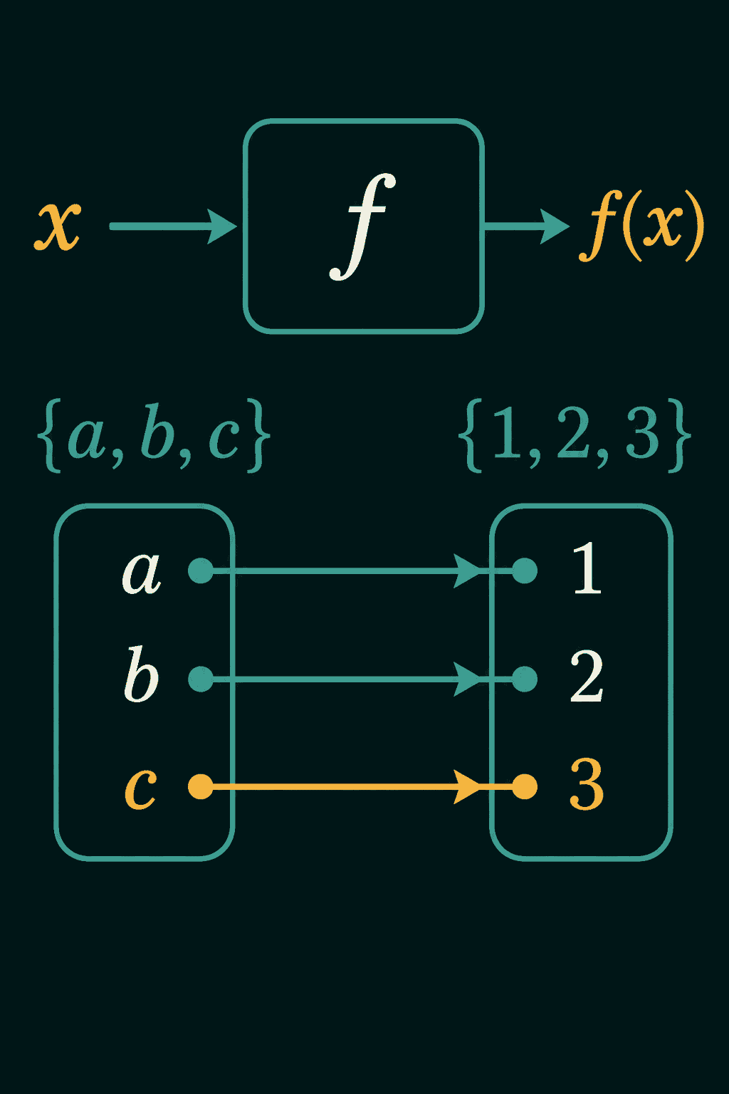
A function takes an input, applies a rule, and returns an output, and the same input always gives the same output. If $f(x) = x^2$, then $f(3) = 9$ every time.

The domain is the set of inputs a function accepts, and the range is the set of outputs it can produce. $f(x) = \sqrt{x}$ has domain $x \geq 0$ if we stay in the real numbers, since a negative input has no real square root, and its range is $y \geq 0$.

A function f drawn as a box taking x and returning f(x), and a mapping from the inputs a, b, c to the outputs 1, 2, 3

Composition: feeding one function into another

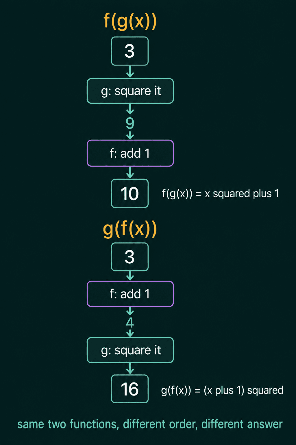
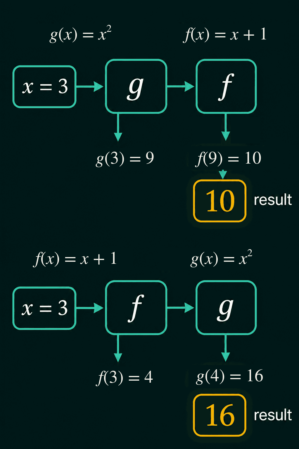
Composition means using the output of one function as the input of another. $f(g(x))$ means compute $g(x)$ first, then pass that result to $f$. The order changes the answer. With $f(x) = x + 1$ and $g(x) = x^2$:

$$f(g(x)) = x^2 + 1$$

$$g(f(x)) = (x+1)^2$$

At $x = 3$, the first gives $9 + 1 = 10$ and the second gives $4^2 = 16$.

Two chains starting from 3: square then add 1 gives 10, add 1 then square gives 16

x equals 3 passed through g then f to give 10, and through f then g to give 16, with g(x) equals x squared and f(x) equals x plus 1

A neural network is a composition. Each layer is a function, and the network is $f_n(f_{n-1}(\cdots f_1(x) \cdots))$, with layer 1 feeding layer 2 and so on.

Inverse functions

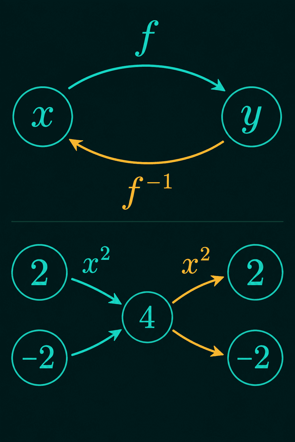
An inverse function, written $f^{-1}$, undoes $f$. If $f(x) = x + 3$, then $f^{-1}(x) = x - 3$, because $f^{-1}(f(x)) = (x + 3) - 3 = x$.

An inverse exists only when $f$ is one-to-one, meaning no two different inputs give the same output. $f(x) = x^2$ over all real numbers fails that test, since $f(2)$ and $f(-2)$ are both 4, so an inverse would not know which input 4 came from. Restricted to $x \geq 0$, it is one-to-one and its inverse is $\sqrt{x}$.

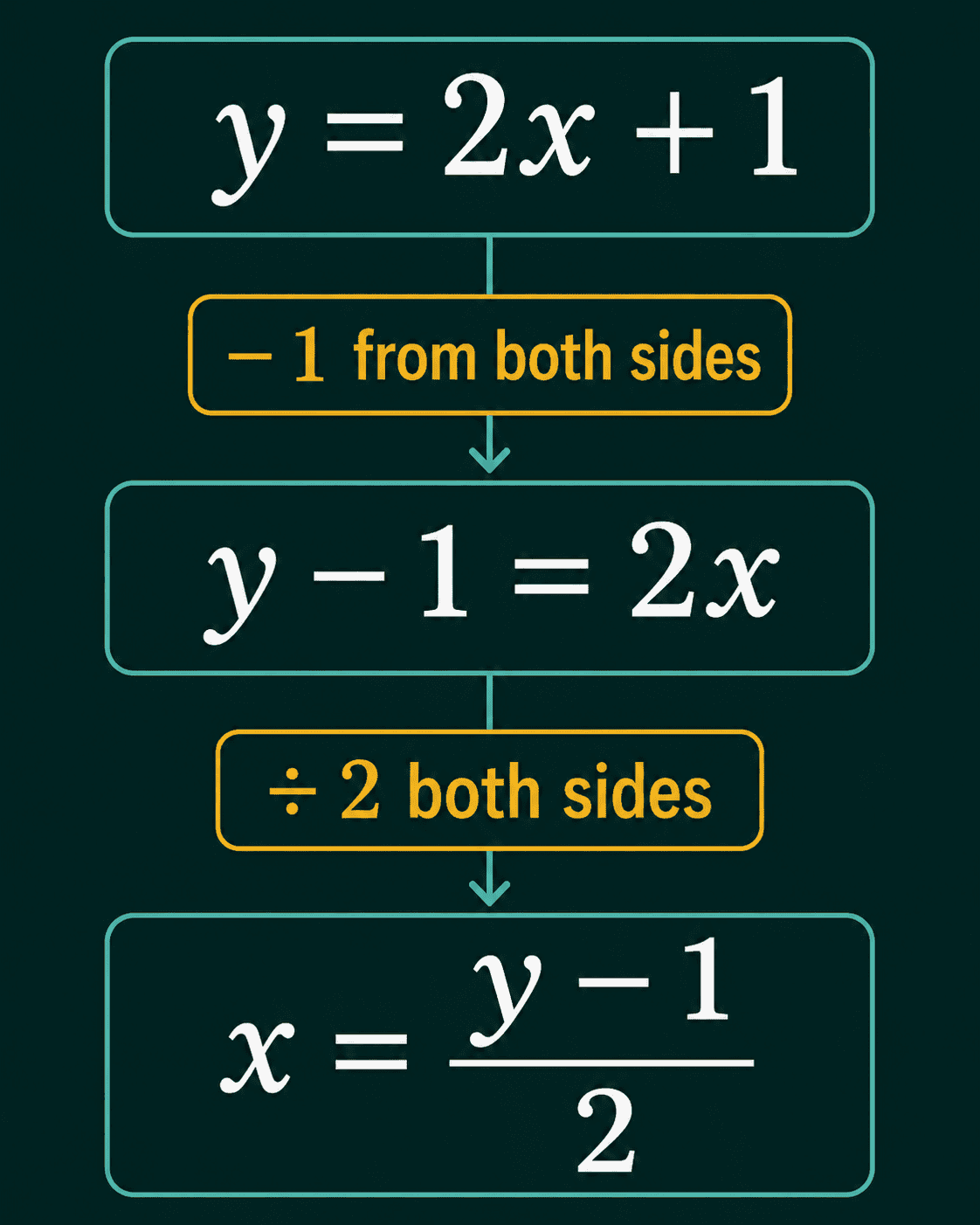
f taking x to y and the inverse taking y back to x, and below, 2 and minus 2 both squaring to 4, so 4 cannot be sent back to a single input

To find an inverse, write $y = f(x)$ and solve for $x$. For $f(x) = 2x + 1$, subtract 1 from both sides to get $y - 1 = 2x$, then divide by 2:

$$f^{-1}(y) = \frac{y - 1}{2}$$

Check it: $f(3) = 7$, and $f^{-1}(7) = 6/2 = 3$.

Solving y equals 2x plus 1 for x: subtract 1 from both sides, then divide both sides by 2, giving x equals y minus 1 over 2

The exponent rules

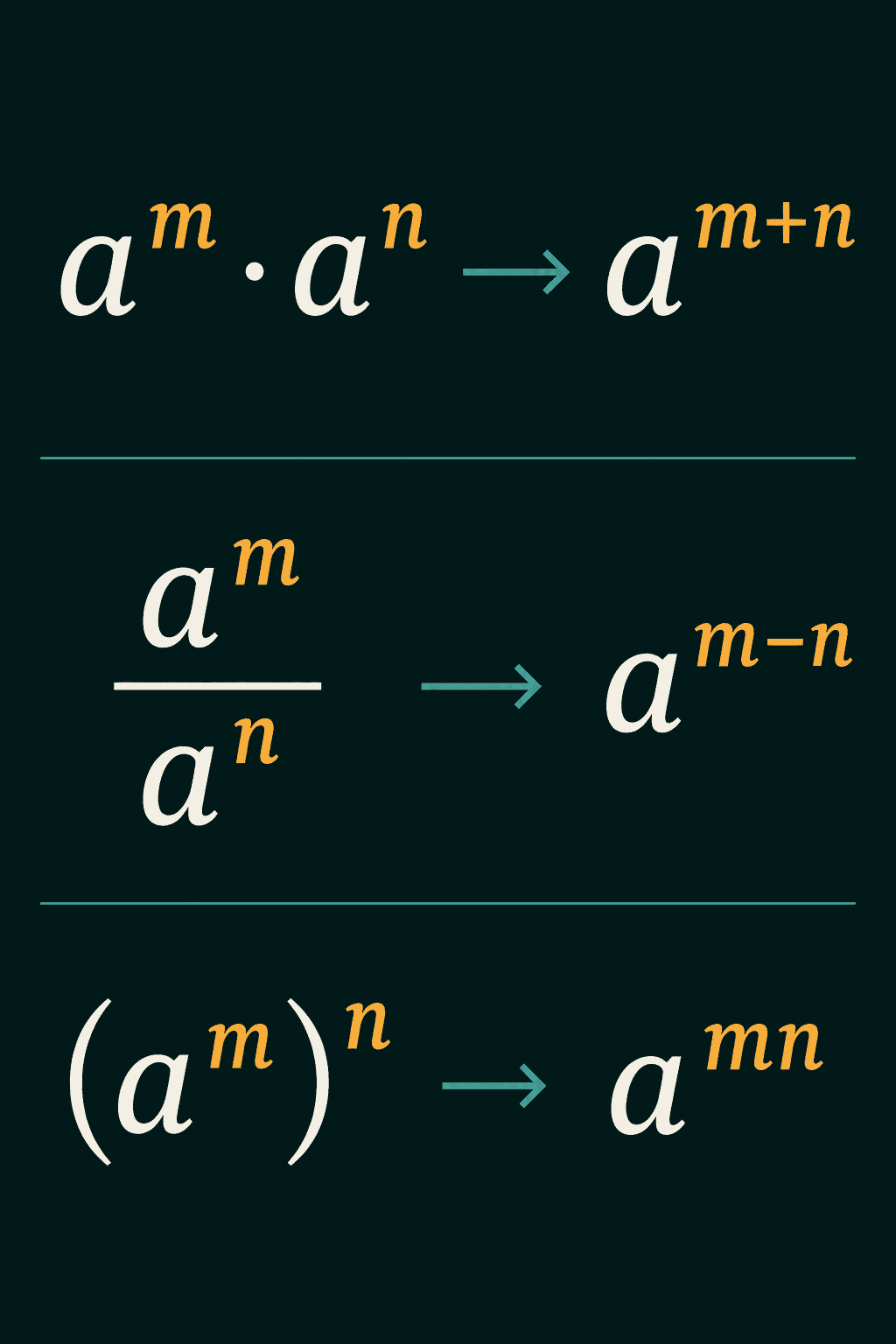
$a^m$ means $a$ multiplied by itself $m$ times, where $a$ is the base and $m$ the exponent. Five rules cover most of what you will meet:

$a^m \cdot a^n = a^{m+n}$, multiplying the same base adds exponents
$a^m / a^n = a^{m-n}$, dividing subtracts them
$(a^m)^n = a^{mn}$, a power of a power multiplies them
$a^{-n} = 1/a^n$, a negative exponent means one over
$a^0 = 1$ for any nonzero $a$

The rules a to the m times a to the n equals a to the m plus n, a to the m over a to the n equals a to the m minus n, and a to the m to the n equals a to the mn

What a logarithm is

A logarithm answers: what power do I raise the base $b$ to, to get $x$?

$$\log_b(x) = y \quad \text{means} \quad b^y = x$$

So $\log_2(8) = 3$ because $2^3 = 8$. In machine learning the base is usually $e \approx 2.718$, and that log is called the natural log, written $\ln(x)$ or $\log(x)$. torch.log is the natural log.

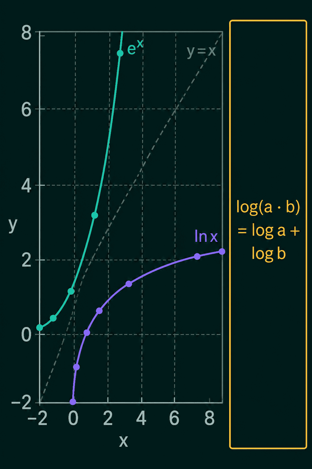
The curve of $\ln(x)$ is the curve of $e^x$ mirrored across the line $y = x$, which is what being inverses looks like on a plot. $\ln(x)$ is only defined for $x > 0$, and it is negative for $0 < x < 1$.

The curves of e to the x and ln x mirrored across the dashed line y equals x, next to the rule log of a times b equals log a plus log b

The log rules

The log rules mirror the exponent rules, because logs and exponents are inverses:

$\log(ab) = \log(a) + \log(b)$, a product becomes a sum
$\log(a/b) = \log(a) - \log(b)$, a quotient becomes a difference
$\log(a^n) = n \log(a)$, a power comes out front

Because log and exp undo each other, $\log(e^x) = x$ and $e^{\log(x)} = x$.

To change base, divide by one log: $\log_b(x) = \ln(x) / \ln(b)$. A base-2 log and a natural log of the same number differ only by a constant factor.

A product of probabilities P1 through Pn turned by a log into a sum of log probabilities, with the log of the product equal to the sum of the logs

Why machine learning works with log-likelihood

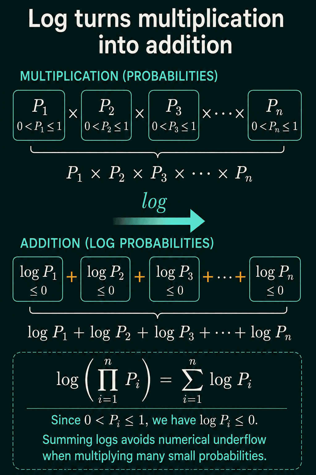
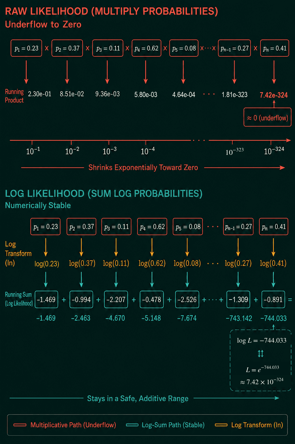
A likelihood is the probability a model assigns to the training data. When the examples are treated as independent, it is the product of one probability per example:

$$L = \prod_{i=1}^{n} p_i$$

Taking the log turns that product into a sum, the log-likelihood:

$$\log L = \sum_{i=1}^{n} \log p_i$$

This helps in two ways. First, gradients of a sum are easy, since you differentiate one term at a time. Second, every $p_i$ is at most 1, so multiplying hundreds of them pushes the product toward zero faster than floating point can follow. Once the true value drops below the smallest number the format can store, the computer rounds it to 0, which is called underflow. The sum of logs is an ordinary negative number that stays easy to store.

The log is an increasing function, so the parameters that make $L$ largest also make $\log L$ largest. Training gets the same optimum with arithmetic that does not underflow. Losses are written to be minimized, so in practice training minimizes the negative log-likelihood, $-\log L$.

The running product of probabilities shrinking from 0.23 to 7.42e-324 and underflowing to 0, next to the running sum of their logs staying at ordinary values down to minus 744.033

Logs in PyTorch

The log rules, checked on $a = 8$ and $b = 4$:

1import torch
2 
3a, b = torch.tensor(8.0), torch.tensor(4.0)
4 
5print(torch.log2(a))                              # 2 to what power is 8?
6print(torch.log(a * b), torch.log(a) + torch.log(b))  # product -> sum
7print(torch.log(a ** 3), 3 * torch.log(a))         # power -> front
8print(torch.log(torch.exp(a)))                    # log undoes exp

1tensor(3.)
2tensor(3.4657) tensor(3.4657)
3tensor(6.2383) tensor(6.2383)
4tensor(8.)

Now 1000 probabilities between 0.05 and 0.95, multiplied directly and then summed as logs:

1import torch
2 
3torch.manual_seed(0)
4probs = torch.rand(1000) * 0.9 + 0.05   # 1000 probabilities between 0.05 and 0.95
5 
6likelihood = probs.prod()
7log_likelihood = torch.log(probs).sum()
8 
9print(likelihood)       # multiply them all
10print(log_likelihood)   # add their logs instead

1tensor(0.)
2tensor(-891.7798)

The true product is about $e^{-891.78}$, far below the smallest number a 32-bit float can hold, so prod() returns exactly 0 and every bit of information in it is gone. The log-likelihood keeps it as -891.78, which a model can compare and take gradients of. If you see a likelihood of exactly 0 in your own code, switch to summing logs first.

Common mistakes with logs

Taking the log of 0. $\log(0)$ is $-\infty$ in PyTorch, and a single one turns a whole sum of logs into $-\infty$ or NaN. A probability that rounds to 0 in floating point is enough to cause it.
Mixing up bases. torch.log is the natural log. torch.log2 and torch.log10 are the base-2 and base-10 versions, and the three differ by a constant factor.
Adding logs of a sum. $\log(a + b)$ is not $\log(a) + \log(b)$. Only a product splits into a sum.
Forgetting the order in a composition. $f(g(x))$ runs $g$ first, the reverse of the reading order.

Summation and product notation is how these formulas are written on paper, with $\Sigma$ for a sum and $\Pi$ for a product. Both are explained in how to read the math notation in ML papers. Sine and cosine are the other functions from this part of the math toolkit that show up in ML features, covered in sine and cosine for machine learning.

QuiddityML teaches exponents and logarithms as their own concept in the Math track, and the exercises include writing log_of_product(a, b) so it never multiplies a * b, ordering the lines of that function, and spotting the bug in a log computation.