By Sagi Shaier · 7 October 2026 · 7 min read

How to read the math notation in ML papers

Machine learning papers write their formulas with a small set of symbols: big sigma and pi, argmin and argmax, hats and bars over letters, a left arrow, and shape declarations like W ∈ ℝ^(m×n). This post explains what each one means and shows the PyTorch line that does the same thing.

Machine learning papers use a lot of math notation, and a handful of the same symbols repeat from paper to paper, each one packing a loop, a search, or a shape into one line. A loss function or a training rule that looks like a wall of symbols usually turns out to be a sum, a search for the best input, and a few labels on top of letters. Once you can read those symbols, most formulas translate straight into a few lines of Python.

This post covers the ones that show up most: $\Sigma$ and $\Pi$, hats, tildes and bars, $\text{argmin}$ and $\text{argmax}$, the update arrow $\leftarrow$, and shape declarations with $\in$.

How to read a sum: the big sigma

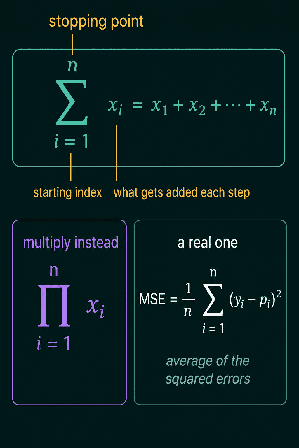
$\Sigma$ (the Greek capital sigma) means "add up a list of things." It has three parts. The index under it says where to start counting, the number on top says where to stop, and the expression to its right is what gets added at each step.

$$\sum_{i=1}^{n} x_i = x_1 + x_2 + \cdots + x_n$$

Read it as: for each $i$ from 1 to $n$, take $x_i$, and add them all together. In code it is a for loop with a running total, or one call to .sum().

The sigma sum with its starting index, stopping point, and the term added each step labeled, next to the product pi and the mean squared error formula

How to read a product: the big pi

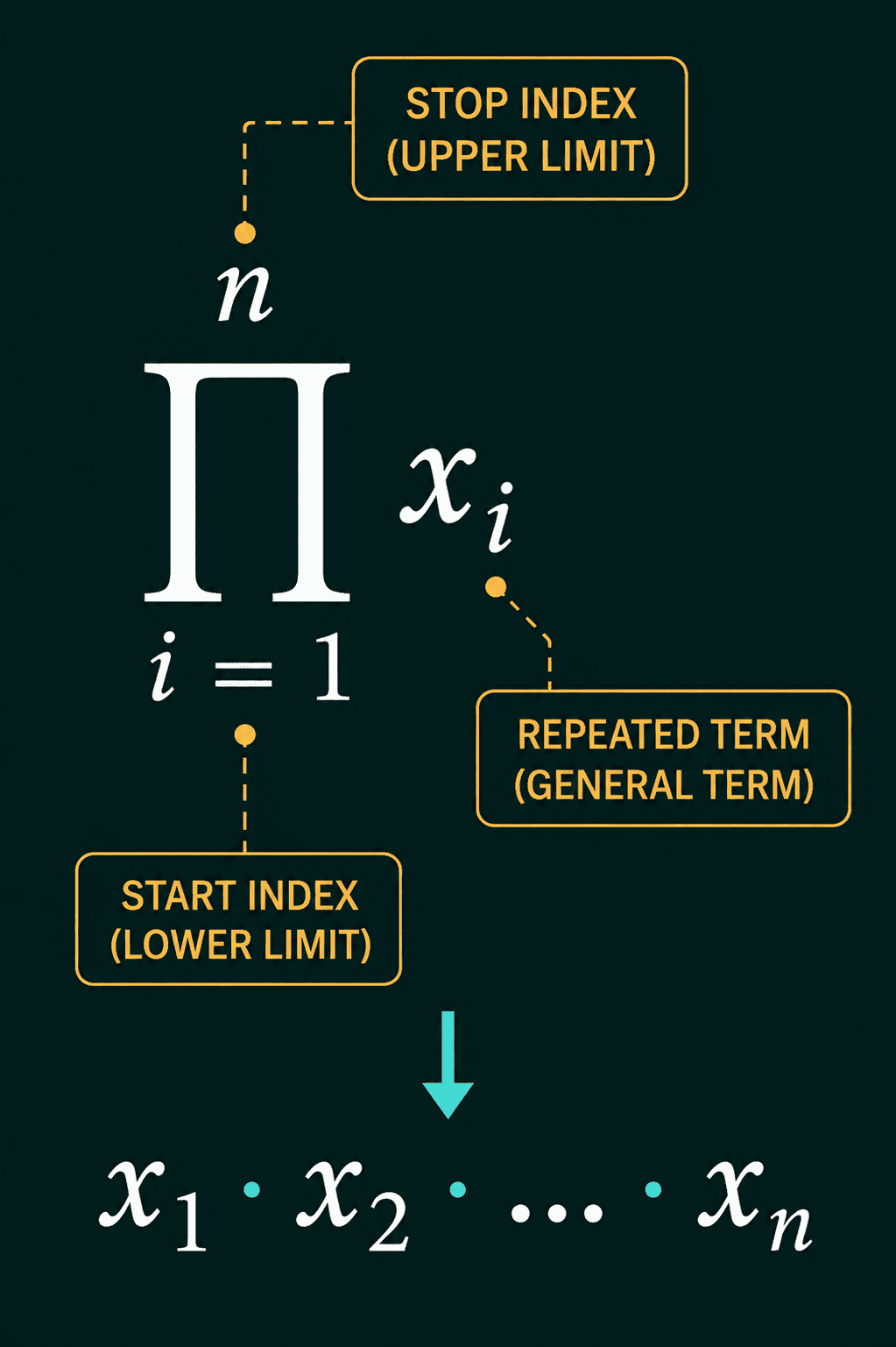
$\Pi$ (capital pi) has the same three parts and multiplies instead of adding:

$$\prod_{i=1}^{n} x_i = x_1 \cdot x_2 \cdots x_n$$

The start index, the stop index, and the repeated term work exactly as in a sum. Products show up most often when a formula multiplies many probabilities together.

The pi product with its start index, stop index, and repeated term labeled, expanding to x1 times x2 up to xn

Nested sums are nested loops

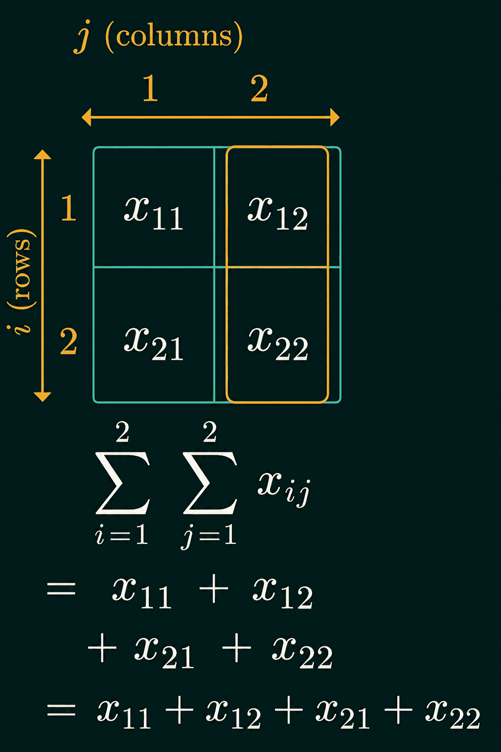
Two sigmas in a row mean a sum inside a sum, one per index. Over a grid with $m$ rows and $n$ columns, where $i$ walks the rows and $j$ walks the columns:

$$\sum_{i=1}^{m} \sum_{j=1}^{n} x_{ij}$$

This reads like a nested for loop: for each row $i$, loop over every column $j$ and add $x_{ij}$. Over a 2 by 2 grid it expands to four terms, $x_{11} + x_{12} + x_{21} + x_{22}$. With the values 1, 2, 3 and 4 in those cells, the total is 10.

A 2 by 2 grid of x values with rows labeled i and columns labeled j, and the double sum expanded into four terms

A real one: mean squared error

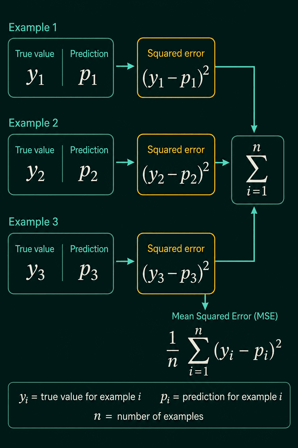
Mean squared error (MSE) is a common loss for models that predict a number. With $y_i$ as the true value for example $i$, $p_i$ as the model's prediction for it, and $n$ as the number of examples:

$$\text{MSE} = \frac{1}{n} \sum_{i=1}^{n} (y_i - p_i)^2$$

For each example, take the difference between the true value and the prediction, square it, add all of those up, and divide by $n$. The whole formula means "average the squared errors."

Three examples, each with a true value and a prediction feeding a squared error box, all summed and divided by n to give the mean squared error

Hats, tildes and bars

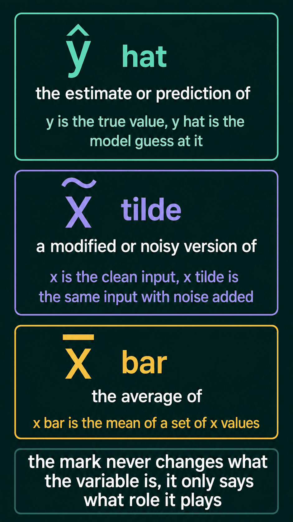
Papers put small marks on top of a letter to say what role that variable plays.

A hat, as in $\hat{y}$ ("y-hat"), means "the estimate or prediction of." $y$ is the true value and $\hat{y}$ is the model's guess at it. The same goes for $\hat{\theta}$, the estimated parameters. The MSE formula above is usually written with $\hat{y}_i$ in place of $p_i$.

A tilde, as in $\tilde{x}$ ("x-tilde"), means "a modified or noisy version of." If $x$ is a clean input, $\tilde{x}$ is the same input with noise added.

A bar, as in $\bar{x}$ ("x-bar"), means "the average of." $\bar{x}$ is the mean of a set of $x$ values.

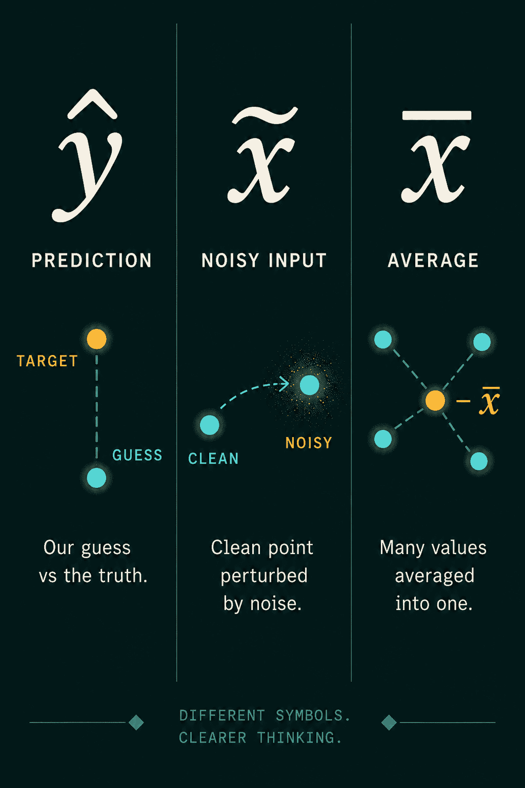
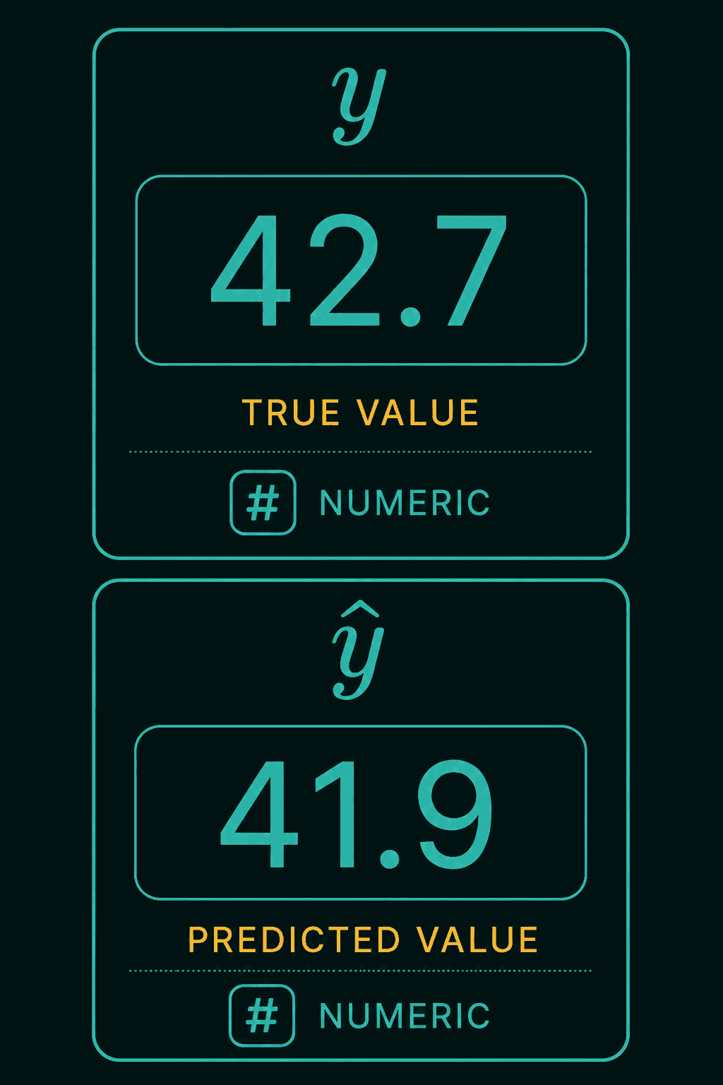
Three panels: y-hat as the estimate or prediction, x-tilde as a noisy version of the input, and x-bar as the average of a set of x values

The prediction as a guess next to a target, a clean point pushed to a noisy point, and several points averaged into one

The marks do not change what kind of thing the variable is. If $y$ is 42.7 and the model predicts 41.9, both $y$ and $\hat{y}$ are plain numbers. The mark only tells you which one is the truth and which one is the guess, and most supervised loss functions compare exactly those two.

y holding the true value 42.7 and y-hat holding the predicted value 41.9, both marked as numeric

Argmin and argmax: the input, not the value

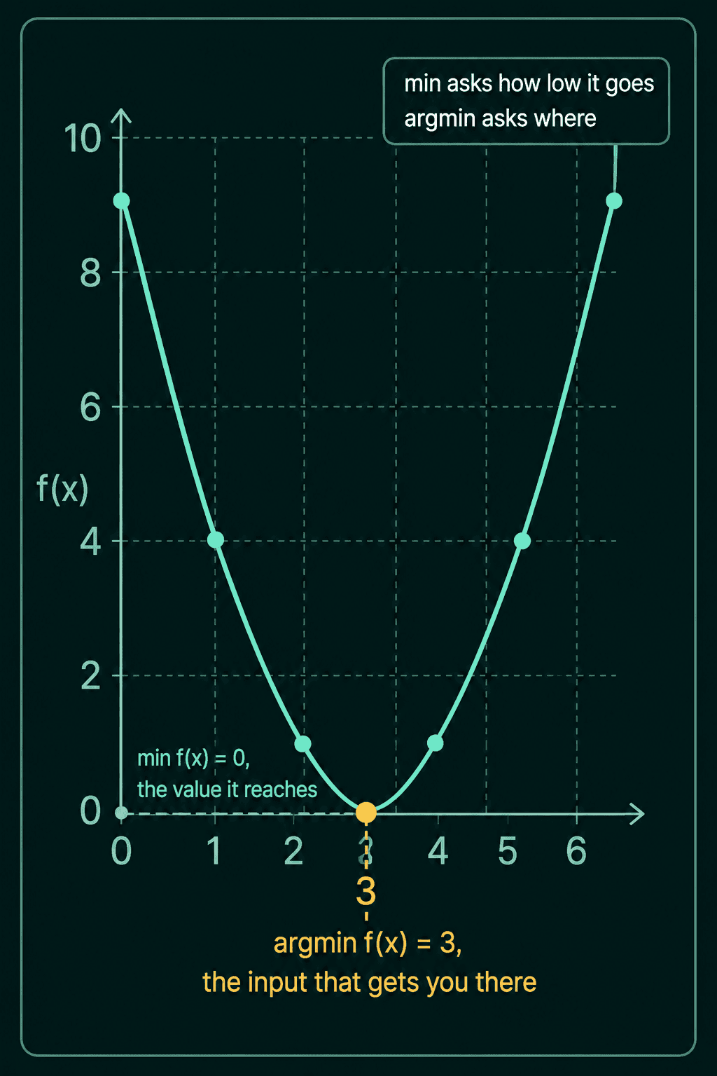
$\min$ and $\max$ give you a value, the smallest or largest number a function or a list produces. $\text{argmin}$ and $\text{argmax}$ give you the input that produced it.

$$\min_x f(x) \quad \text{vs.} \quad \text{argmin}_x f(x)$$

Take $f(x) = (x-3)^2$. Its minimum value is 0, since a squared term never goes below 0. $\text{argmin}_x f(x)$ is 3, because $x = 3$ is the input that makes $f(x)$ equal 0. $\min$ says how low the function goes, and $\text{argmin}$ says where.

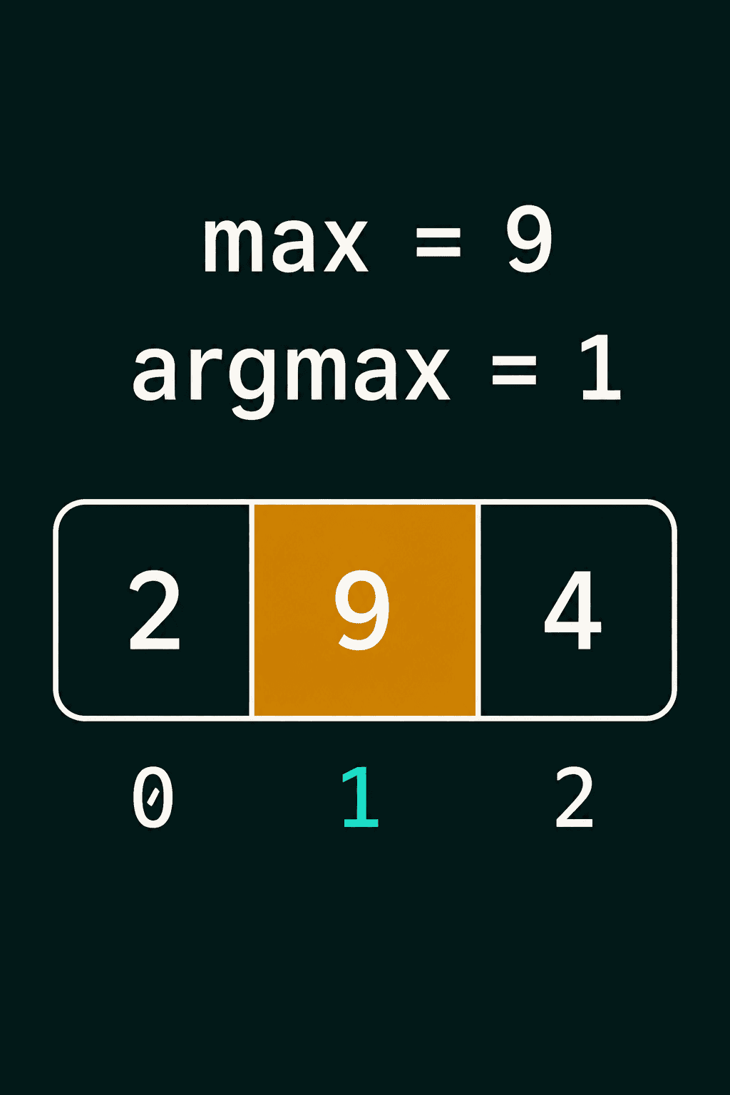
A parabola with its lowest point at x equals 3, labeled min f(x) equals 0 for the value and argmin f(x) equals 3 for the input

Over a list, the answer is a position. For $[2, 9, 4]$, the max is 9 and the argmax is 1, the index of the 9 when counting from 0.

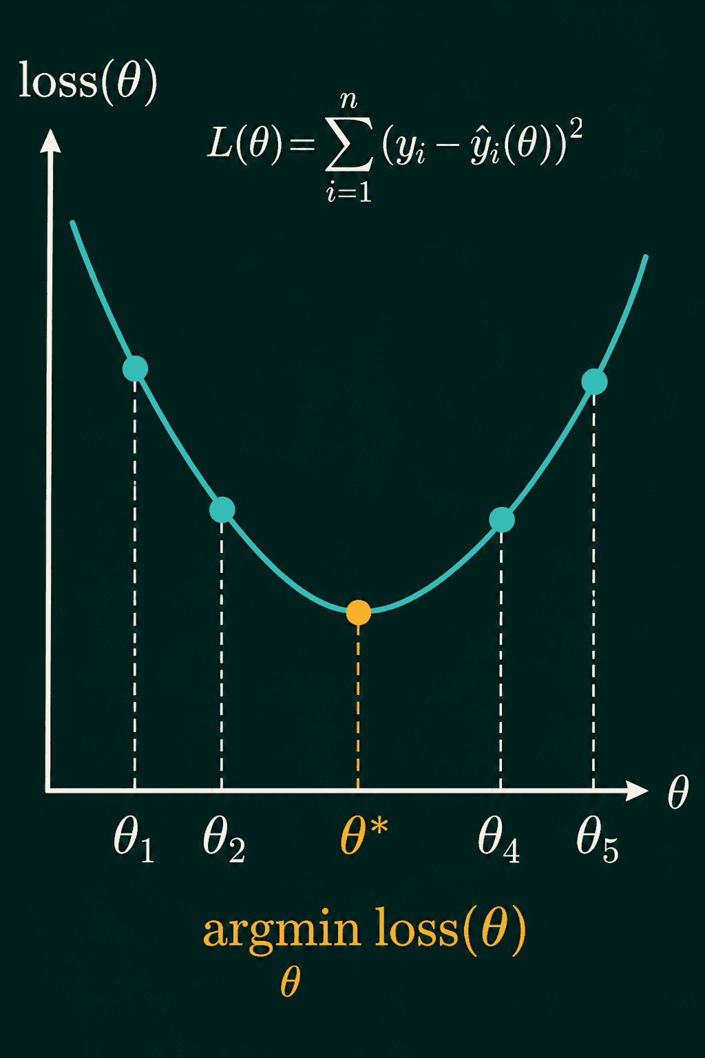
The list 2, 9, 4 with the 9 highlighted at index 1, showing max equals 9 and argmax equals 1

This is also how training is written. In optimization formulas, $\theta$ usually stands for the model's parameters (in trigonometry the same letter is an angle). $f_\theta(x_i)$ is the model's prediction for input $x_i$ using parameters $\theta$, so the training goal reads:

$$\text{best } \theta = \text{argmin}\theta \sum{i=1}^{n} (y_i - f_\theta(x_i))^2$$

Search over possible values of $\theta$, compute the total squared error each one gives, and return the $\theta$ with the smallest total. The picture below writes the prediction as $\hat{y}_i(\theta)$ and labels the best value $\theta^*$, a common name for the argmin.

A loss curve over theta with five candidate values, the lowest point labeled theta star, and argmin of the loss written underneath

The update arrow means overwrite

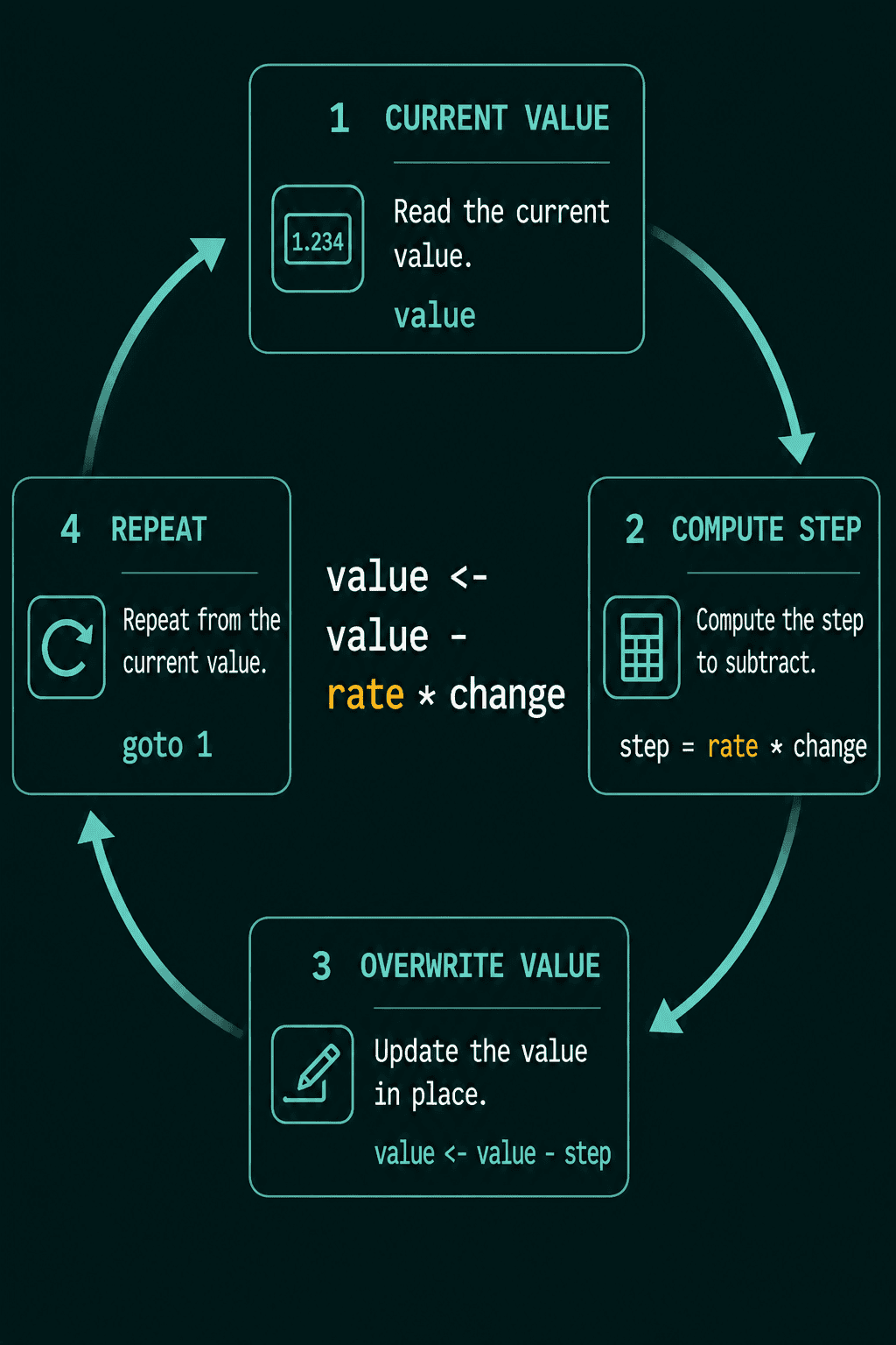
The left arrow $\leftarrow$ marks reassignment:

$$x \leftarrow x + 1$$

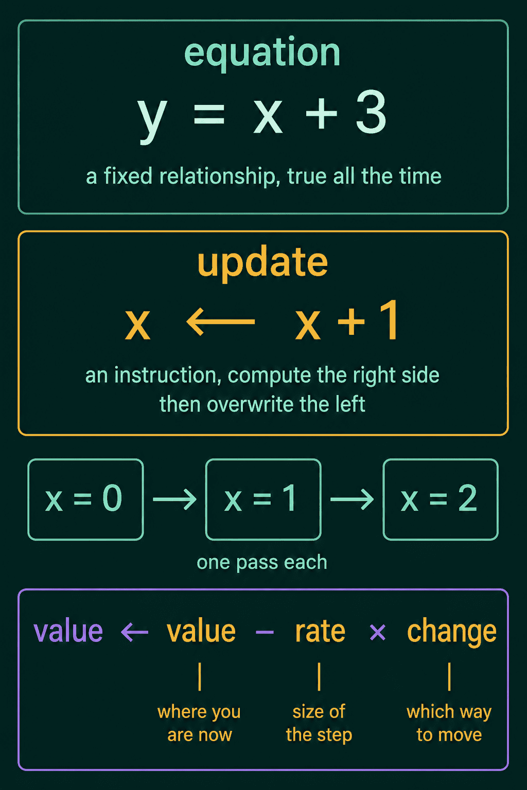
Read it as "gets reassigned to." An equation like $y = x + 3$ states a relationship that holds all the time. $x = x + 1$ as an equation would be false for every number, so the arrow is there to say this line is an instruction: take the current $x$, add 1, and store the result back in $x$. It means the same thing as x = x + 1 in Python.

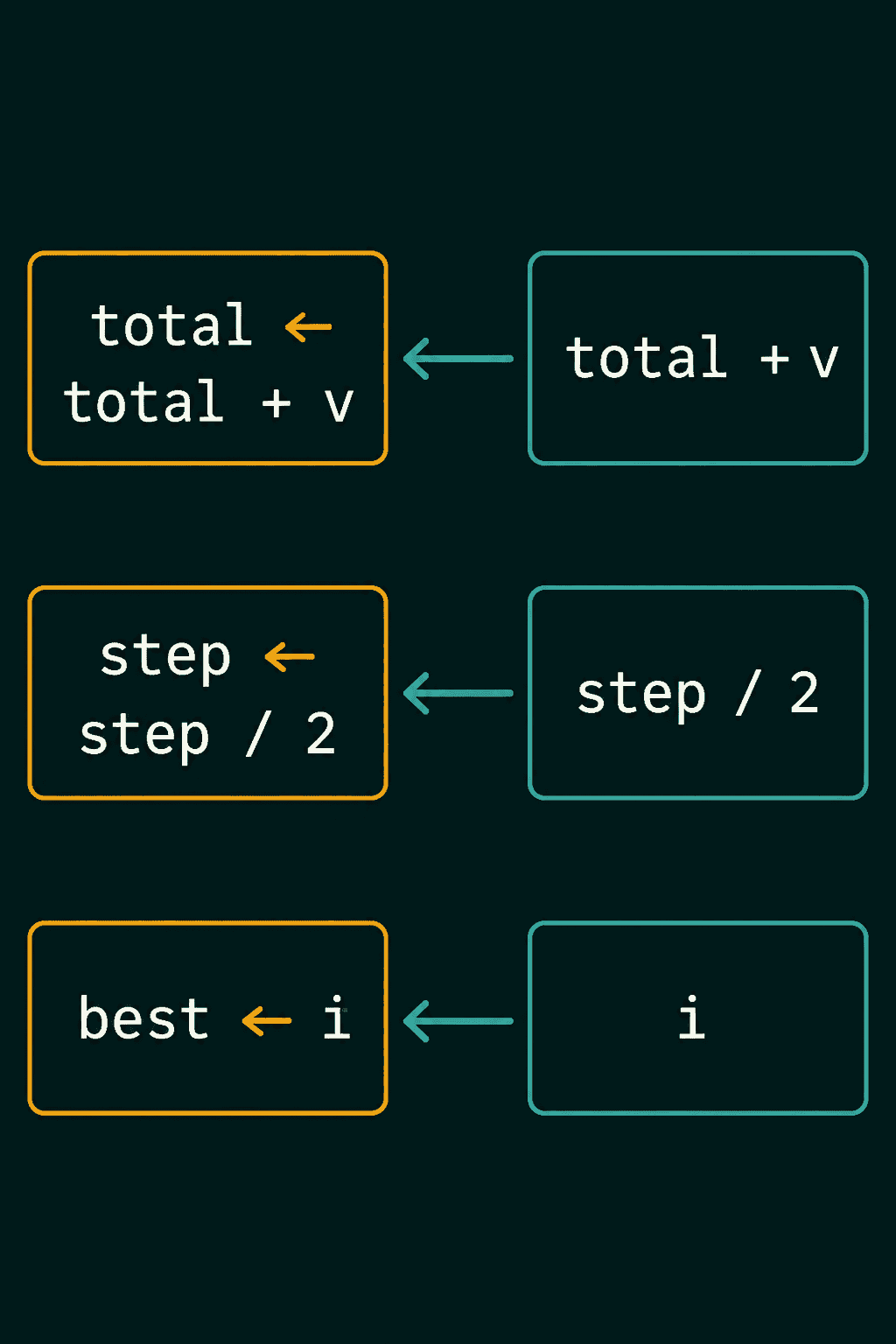
An equation y equals x plus 3 next to the update x gets x plus 1, with x stepping from 0 to 1 to 2, and the update value gets value minus rate times change

A few more that only make sense as instructions: $\text{total} \leftarrow \text{total} + v$ adds $v$ to a running total, $\text{step} \leftarrow \text{step} / 2$ halves a step size, and $\text{best} \leftarrow i$ records $i$ as the new best. Each one computes the right-hand side from the current values, then overwrites the left side.

Three updates: total gets total plus v, step gets step divided by 2, and best gets i

The shape you will meet most is:

$$\text{value} \leftarrow \text{value} - \text{rate} \times \text{change}$$

Start from the current value, move it by an amount, overwrite it, and repeat. The rate sets how big each move is. Gradient descent, the method behind most model training, is this line repeated with a specific choice of change, and the arrow tells you the line is a step you run many times.

A loop of four steps: read the current value, compute the step as rate times change, overwrite the value, and repeat

Set membership and shapes

The symbol $\in$ means "is a member of." $\mathbb{R}$ is the set of all real numbers, so $x \in \mathbb{R}$ reads "x is a real number."

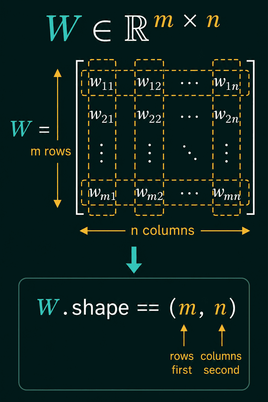
A superscript on $\mathbb{R}$ declares a shape. $x \in \mathbb{R}^d$ says $x$ is a vector of $d$ real numbers. $W \in \mathbb{R}^{m \times n}$ says $W$ is a matrix with $m$ rows and $n$ columns, and the rows always come first.

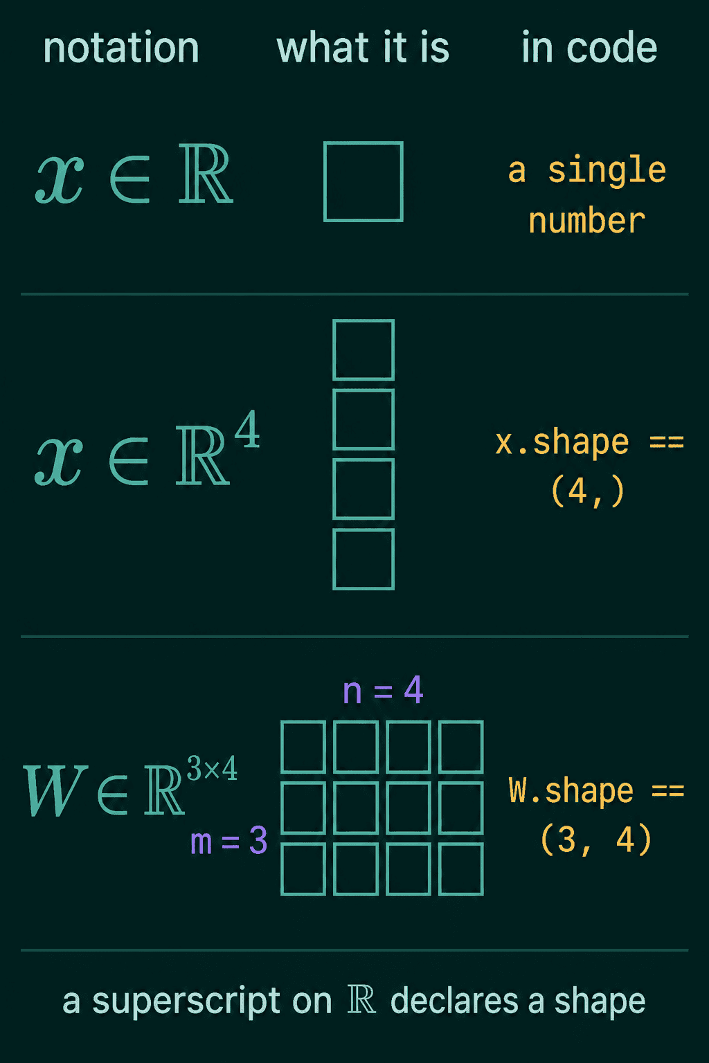
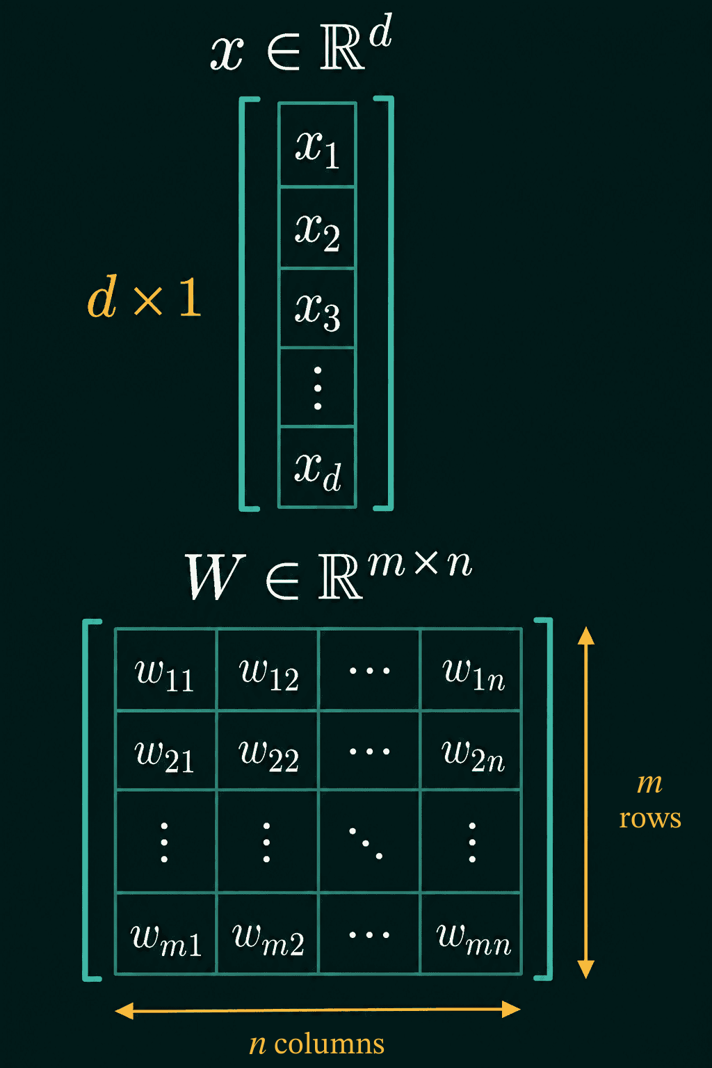
A table of notation, picture, and code: x in R as a single number, x in R4 as four boxes with shape (4,), and W in R 3 by 4 as a grid with shape (3, 4)

A d-dimensional vector drawn as a column of d entries, and an m by n matrix W with its m rows and n columns labeled

The same fact appears in code as a shape check: the math says $W \in \mathbb{R}^{m \times n}$ and PyTorch says W.shape == (m, n). A plain scalar $s \in \mathbb{R}$ has no dimensions, so its shape is the empty tuple (), not (1,).

W in R m by n translating to W.shape equals (m, n), with rows first and columns second

The same symbols in PyTorch

Most of these symbols map to one PyTorch call or one line of Python. On the list $[2, 9, 4]$:

1import torch
2 
3x = torch.tensor([2.0, 9.0, 4.0])
4 
5print(x.sum())       # sigma: 2 + 9 + 4
6print(x.prod())      # pi: 2 * 9 * 4
7print(x.max(), x.argmax())   # the value, and where it is
8print(x.mean())      # x-bar, the average

1tensor(15.)
2tensor(72.)
3tensor(9.) tensor(1)
4tensor(5.)

Mean squared error with $y$ and $\hat{y}$, written the way the formula reads:

1import torch
2 
3y = torch.tensor([3.0, 5.0, 2.0])       # true values
4y_hat = torch.tensor([2.5, 5.5, 2.0])   # predictions
5 
6n = y.shape[0]
7mse = ((y - y_hat) ** 2).sum() / n
8print(mse)

1tensor(0.1667)

The squared errors are 0.25, 0.25 and 0, which add to 0.5, and 0.5 divided by 3 is 0.1667.

Argmin over a grid of candidate inputs for $f(x) = (x-3)^2$:

1import torch
2 
3f = lambda x: (x - 3) ** 2
4xs = torch.linspace(0, 6, 61)   # candidate inputs 0.0, 0.1, ..., 6.0
5values = f(xs)
6 
7print(values.min())          # min: how low it goes
8print(xs[values.argmin()])   # argmin: where

1tensor(0.)
2tensor(3.)

The update arrow is a reassignment inside a loop. Here the change is $2 \times \text{value}$, which pulls the value toward 0:

1value = 10.0
2rate = 0.1
3for step in range(3):
4    change = 2 * value            # how the value should move this step
5    value = value - rate * change # value <- value - rate * change
6    print(step, value)

10 8.0
21 6.4
32 5.12

And shape declarations become shapes:

1import torch
2 
3d, m, n = 4, 3, 4
4x = torch.zeros(d)      # x in R^d
5W = torch.zeros(m, n)   # W in R^(m x n)
6s = torch.tensor(2.5)   # s in R
7 
8print(x.shape, W.shape, s.shape)
9assert W.shape == (m, n)

1torch.Size([4]) torch.Size([3, 4]) torch.Size([])

If a translation gives a different number than you expect, check the index range first: papers usually count from 1, and Python counts from 0.

Common mistakes when reading notation

Reading the arrow as an equals sign. $\text{value} \leftarrow \text{value} - \text{rate} \times \text{change}$ is a step that runs again and again, not a fact about the value.
Mixing up max and argmax. A classifier's predicted class is the argmax of its scores (a position), not the max (a score).
Reading $\mathbb{R}^{m \times n}$ as columns first. Rows come first in the notation and in W.shape.
Treating $\hat{y}$ as a different kind of object from $y$. Both are the same kind of number, one true and one predicted.
Off-by-one indexes. $\sum_{i=1}^{n}$ in a paper is range(n) or x[0:n] in Python.

Exponents and logarithms sit inside many of these formulas, especially $\log$ wrapped around a product, which turns a $\Pi$ into a $\Sigma$. That gets its own post in exponents and logarithms for machine learning. $\theta$ has a second life as an angle in sine and cosine for machine learning, where it is the input to $\sin$ and $\cos$.

QuiddityML teaches each of these symbols as its own concept in the Math track, and the exercises include turning a sigma into a line of PyTorch, putting the lines of a mean squared error function in order, and translating a paper's shape declarations into code shapes.