17 September 2026 · optimizersml-foundation
Machine learning optimizers explained: SGD, momentum, RMSProp, Adam, AdamW
An optimizer is the rule that turns gradients into parameter updates. This post explains the five optimizers most models train with, in the order each one was invented to fix the last, and which one to pick.
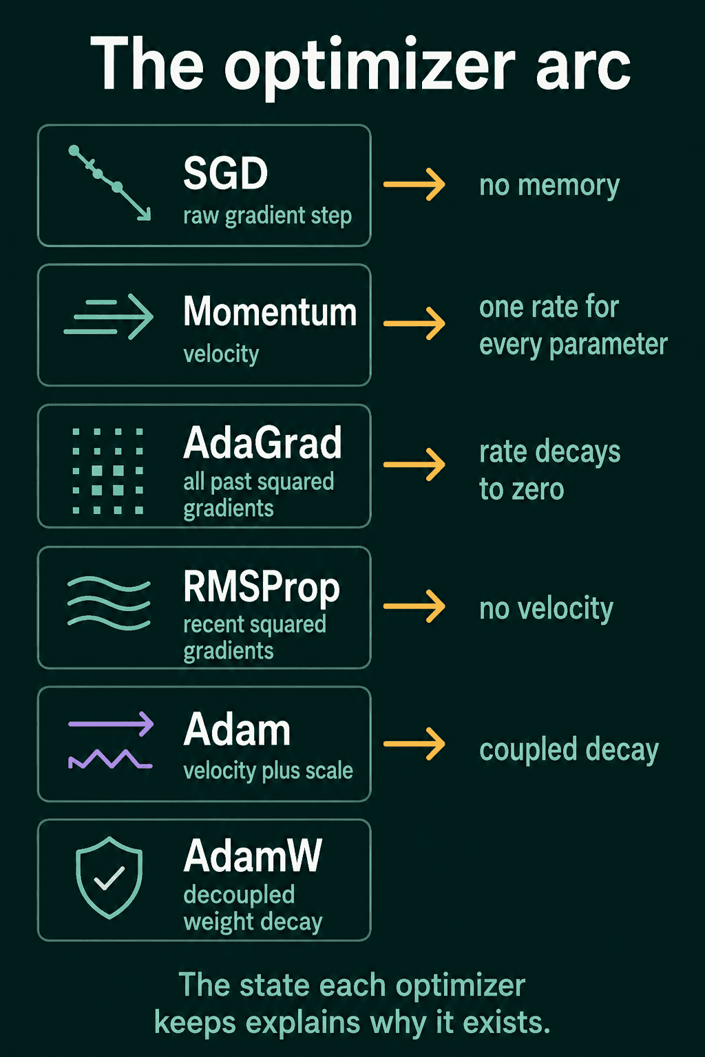
An optimizer is the rule that decides how much to change each parameter of a model after every training step. Training computes a loss, the loss produces a gradient for every parameter, and the optimizer turns that gradient into an update. Most people pick one from a dropdown and never think about it again, which is fine until training stalls or blows up and every optimizer has different knobs. This post goes through the five you will meet most often, in the order each one was built to fix a problem with the one before, so the names stop being a list to memorize.
What every optimizer has in common
A training step has three parts. The model makes predictions on a batch of examples and a loss function scores how wrong they are. Backpropagation computes the gradient, which is one number per parameter saying which direction, and how steeply, the loss goes up if that parameter grows. The optimizer then moves each parameter a small distance the other way. Every optimizer in this post follows that loop and differs only in how it converts the gradient into a step. In PyTorch the loop looks the same no matter which one you use:
1for x, y in loader:
2    optimizer.zero_grad()
3    loss = loss_fn(model(x), y)
4    loss.backward()
5    optimizer.step()
SGD: the plain step
Stochastic gradient descent is the baseline. Call the parameters $\theta$, the gradient of the loss $\nabla L$, and the learning rate $\eta$, a small positive number you choose that scales every step. The update is
$$\theta \leftarrow \theta - \eta \cdot \nabla L$$
Move every parameter against its gradient, scaled by one shared learning rate. The "stochastic" part means the gradient is computed on a mini-batch of 32 to 512 examples instead of the whole dataset, which is cheaper per step and adds noise that in practice helps training avoid sharp, poorly generalizing regions of the loss.
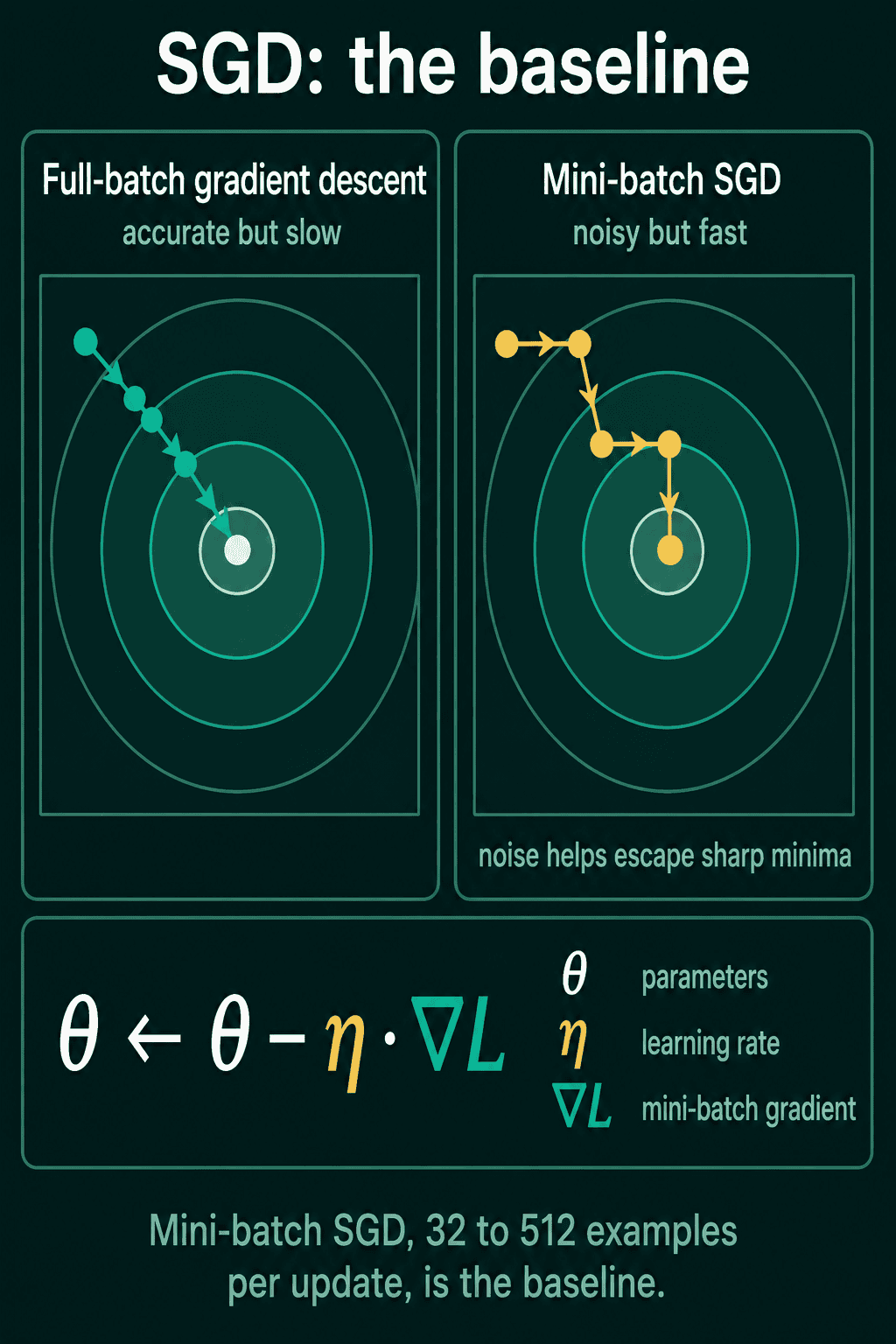
Plain SGD has two weaknesses. It has no memory, so on a loss surface shaped like a long narrow valley it bounces from wall to wall while creeping slowly along the floor. And it uses one learning rate for every parameter, even though a parameter that gets huge gradients and one that gets tiny gradients would each want a different step size.
Momentum: keep a velocity
Momentum fixes the bouncing. Instead of stepping along the current gradient, the optimizer keeps a running velocity $v$ that accumulates past gradients, and steps along that. With $\beta$ controlling how much of the old velocity survives each step (0.9 is the usual default),
$$v \leftarrow \beta v + \nabla L \qquad \theta \leftarrow \theta - \eta \cdot v$$
When consecutive gradients point the same way the velocity grows, so progress along the valley floor speeds up. When they alternate sign, as they do across the valley walls, they cancel inside $v$ and the bouncing shrinks.
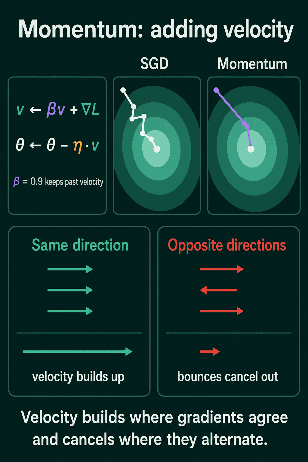
Momentum still uses one learning rate for every parameter, which is the second weakness.
AdaGrad and RMSProp: a step size per parameter
AdaGrad was the first common answer. It keeps, for every parameter, the sum of all its past squared gradients and divides the learning rate by the square root of that sum. A parameter that has seen large gradients gets smaller steps, a parameter that has seen small ones gets larger steps. The flaw is that the sum only grows, so every effective learning rate shrinks toward zero and training stops making progress whether or not it has finished.
RMSProp keeps the idea and fixes the decay. Instead of a lifelong sum it keeps an exponential moving average of the squared gradient, which means a running average that weights recent values more than old ones. Writing the current gradient as $g_t$, the average as $v_t$, and a small constant $\varepsilon$ that only stops division by zero,
$$v_t = \beta v_{t-1} + (1 - \beta), g_t^2 \qquad \theta \leftarrow \theta - \frac{\eta}{\sqrt{v_t} + \varepsilon} \cdot g_t$$
Because old squared gradients fade out, the effective step size can recover when recent gradients get small.
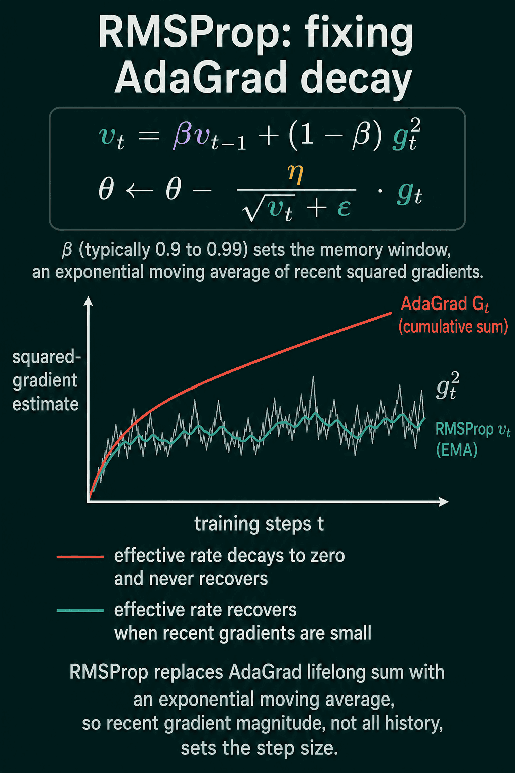
RMSProp gives each parameter its own scale but has no velocity, so it does not get momentum's help in narrow valleys.
Adam: momentum and RMSProp together
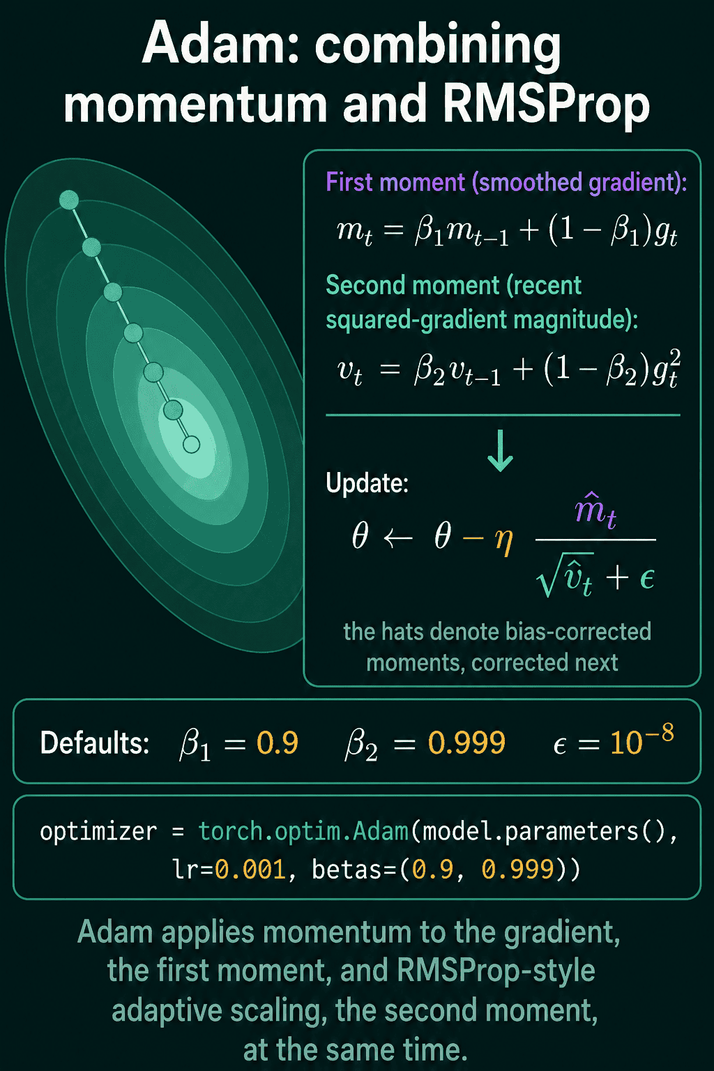
Adam keeps both running averages. The first, $m_t$, is a moving average of the gradient itself, which is momentum. The second, $v_t$, is the moving average of the squared gradient from RMSProp. Each has its own decay rate, $\beta_1$ for $m_t$ and $\beta_2$ for $v_t$:
$$m_t = \beta_1 m_{t-1} + (1 - \beta_1), g_t \qquad v_t = \beta_2 v_{t-1} + (1 - \beta_2), g_t^2$$
Both averages start at zero, so for the first few steps they are much smaller than the gradients they are averaging, and the updates would be far too timid. Adam divides each by a correction factor that is large early and fades to one, written $\hat m_t$ and $\hat v_t$, then updates with
$$\theta \leftarrow \theta - \eta \frac{\hat m_t}{\sqrt{\hat v_t} + \varepsilon}$$
The defaults, $\beta_1 = 0.9$, $\beta_2 = 0.999$, and a learning rate around $10^{-3}$, work on a wide range of problems, which is why Adam became the usual first choice. The full derivation, including why the correction factors have the form they do, is in the Adam post.
AdamW: fix weight decay
Weight decay shrinks every parameter a little on each step to keep the model from relying on huge weights, which helps it generalize. The traditional way to get it is to add an L2 penalty to the loss, which shows up as an extra term in the gradient. Under SGD that is exactly weight decay. Under Adam it is not, because the extra gradient term gets divided by $\sqrt{\hat v_t}$ like everything else, so parameters with large gradients barely decay at all. AdamW moves the decay out of the gradient and applies it directly to the parameters, after the Adam step, with its own coefficient $\lambda$:
$$\theta \leftarrow \theta - \eta \left( \frac{\hat m_t}{\sqrt{\hat v_t} + \varepsilon} + \lambda \theta \right)$$
That is the whole change, and it is why torch.optim.AdamW with weight_decay=0.01 is the default in most transformer recipes while torch.optim.Adam with the same argument behaves differently.
Which one to use
| Situation | Start with | Settings |
|---|---|---|
| New experiment | AdamW | lr=1e-3 (3e-4 for transformers), weight_decay=0.01 |
| CNN on images, tuned schedule | SGD + momentum | lr=0.1, momentum=0.9, weight_decay=5e-4 |
| AdamW stuck on validation | SGD + momentum, as a comparison | same as the row above |
| RMSProp | rarely on its own now | lr=1e-3, alpha=0.99 |
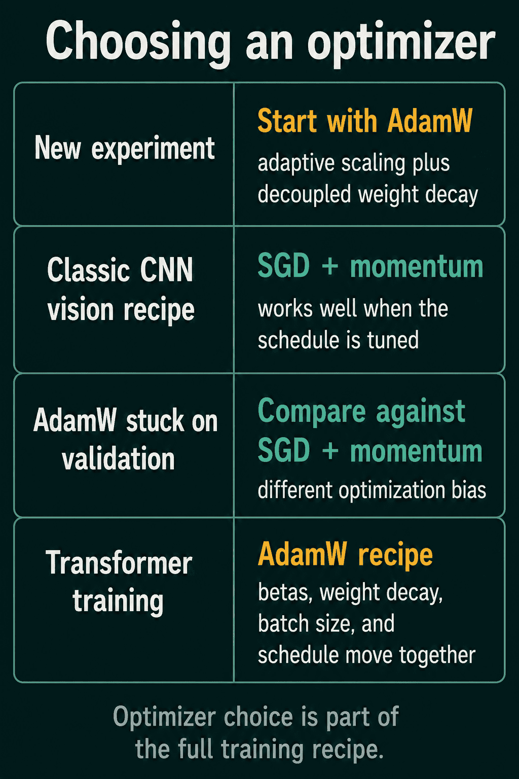
The learning rates are not interchangeable. A good SGD learning rate is often 10 to 100 times larger than a good Adam one, because Adam's division by $\sqrt{\hat v_t}$ already normalizes the step size.
1import torch
2
3sgd   = torch.optim.SGD(model.parameters(), lr=0.1, momentum=0.9, weight_decay=5e-4)
4rms   = torch.optim.RMSprop(model.parameters(), lr=1e-3, alpha=0.99)
5adam  = torch.optim.Adam(model.parameters(), lr=1e-3, betas=(0.9, 0.999))
6adamw = torch.optim.AdamW(model.parameters(), lr=1e-3, weight_decay=0.01)
If the loss is flat or explodes, change the learning rate first, by a factor of 10 in each direction, before touching anything else.
Common mistakes
- Forgetting
optimizer.zero_grad(). PyTorch adds new gradients onto the old ones, so without it every step uses the sum of all gradients so far and training goes wrong quietly. - Reusing Adam's learning rate for SGD, or the reverse. Adam at 0.1 diverges, SGD at 0.001 crawls.
- Passing
weight_decaytoAdamand expecting weight decay. That is the coupled L2 version described above. UseAdamW. - Dropping optimizer state when resuming from a checkpoint. Momentum, RMSProp, Adam, and AdamW all carry running averages, and a checkpoint that saves only the model weights throws them away. On resume the averages restart at zero, which for Adam means a few steps of overcorrected updates and a visible loss spike. Save and load
optimizer.state_dict()next to the model's. Plain SGD has no state, so this is the one optimizer where it does not matter. - Switching optimizers mid-training and keeping the old learning rate. The scale of a good step changes with the optimizer, so retune it.
Related concepts
The learning rate is the one setting shared by all five, and what happens when it is too small or too large is its own topic in the learning rate post. Learning rate schedules, such as warmup and cosine decay, change $\eta$ over the course of training and are used with any of these optimizers. Gradient clipping caps the size of the gradient before the optimizer sees it and is a separate safeguard against exploding updates.
QuiddityML teaches these as one arc of concepts in the ML Foundation track, from SGD through AdamW, and each one has an exercise where the reader writes the optimizer from scratch in PyTorch from its equation, plus a spot-the-bug exercise on a training loop that never zeroes its gradients. What was hard comes back sooner in review, and what was easy stays away (quiddityml.com).