By Sagi Shaier · 26 October 2026 · 6 min read
How to handle class imbalance in text classification
Why a spam filter can score 98% accuracy while catching no spam, which numbers to report instead, and how reweighting, oversampling and undersampling work in PyTorch, with what each one costs.
Class imbalance is when some labels appear far more often than others in a dataset. Spam filtering is a common case: most of a normal inbox is legitimate mail and only a small slice is spam. The rare class is usually the one the model was built to find, so a model that ignores it can look good on paper and fail at its only job.
Why accuracy misleads
Accuracy is the share of predictions that are correct. Picture an inbox where 98% of messages are legitimate and 2% are spam. A model that labels every message "legitimate" without reading it is right 98 times out of 100, and it has never caught a spam email.
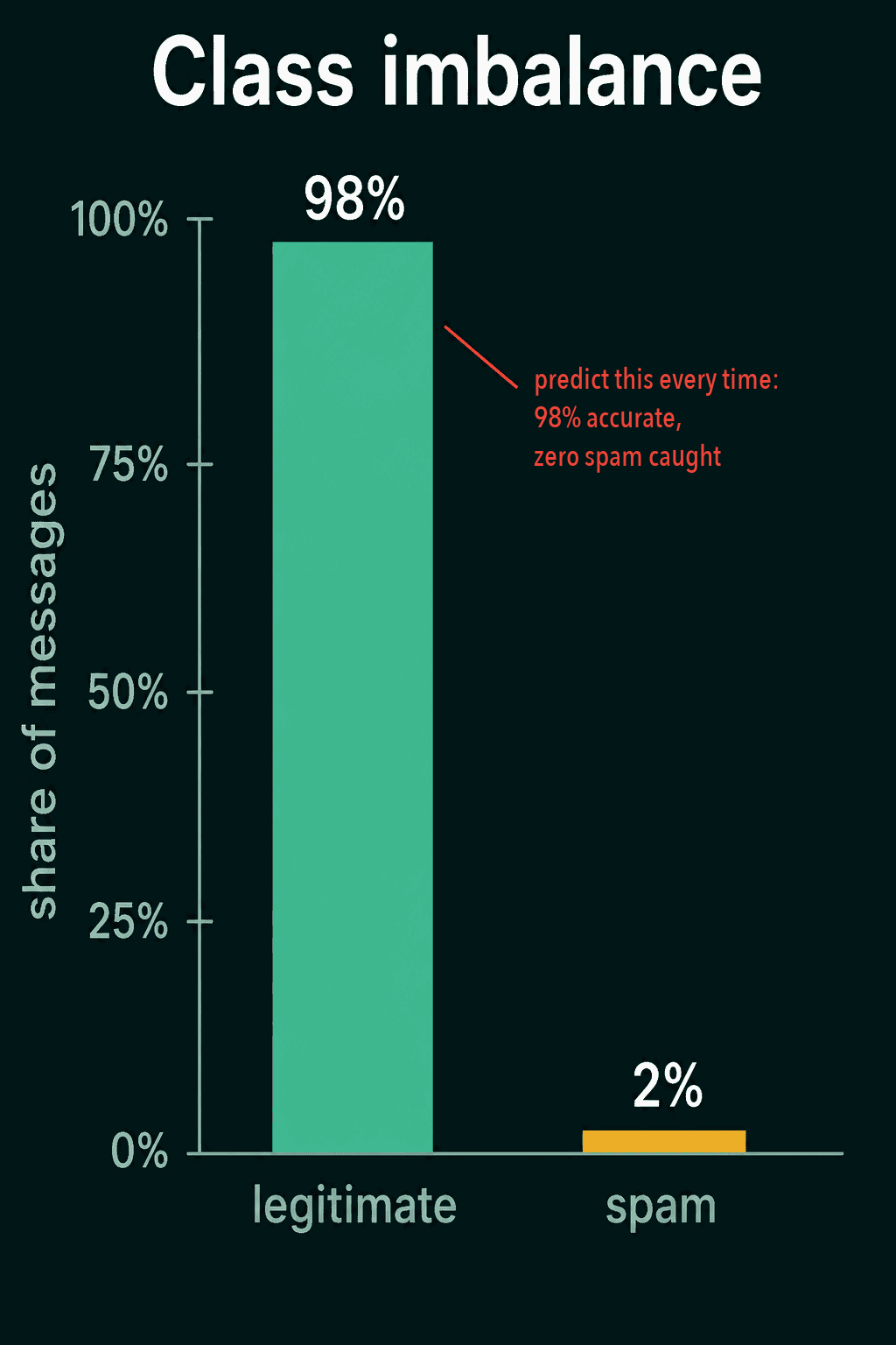
The larger the majority class, the higher this do-nothing accuracy goes. On imbalanced data, accuracy mostly measures how common the majority class is.
Metrics that look at the rare class
The fix is to report numbers computed on the class you care about. For the spam class, every prediction falls into one of four groups:
- TP (true positive): spam the model flagged as spam.
- FP (false positive): legitimate mail the model flagged as spam.
- FN (false negative): spam the model missed.
- TN (true negative): legitimate mail the model left alone.
Precision is the share of flagged messages that were spam:
$$\text{precision} = \frac{TP}{TP + FP}$$
Recall is the share of all spam that the model caught:
$$\text{recall} = \frac{TP}{TP + FN}$$
F1 combines the two with a harmonic mean, which stays low unless both are decent:
$$F1 = \frac{2 \times \text{precision} \times \text{recall}}{\text{precision} + \text{recall}}$$
Here are all four numbers in one function. Each division is guarded, since a model that flags nothing has $TP + FP = 0$:
1def classification_metrics(tp, fp, fn, tn):
2    accuracy = (tp + tn) / (tp + fp + fn + tn)
3    precision = tp / (tp + fp) if tp + fp else 0
4    recall = tp / (tp + fn) if tp + fn else 0
5    f1 = 2 * precision * recall / (precision + recall) if precision + recall else 0
6    return accuracy, precision, recall, f1
7
8# 1,000 messages, 20 of them spam
9print(classification_metrics(tp=0, fp=0, fn=20, tn=980))   # (0.98, 0, 0.0, 0)
10print(classification_metrics(tp=15, fp=10, fn=5, tn=970))  # (0.985, 0.6, 0.75, 0.6666666666666665)
The first line is the always-legitimate model on 1,000 messages with 20 spam. It catches none of the spam, so recall and F1 are 0 while accuracy reads 98%.
The second line is a model that flags 25 messages, 15 of which are spam. Precision is $15 / 25 = 0.6$ and recall is $15 / 20 = 0.75$, giving an F1 of about 0.67. Its accuracy is 98.5%, only half a point above the model that does nothing. Recall and F1 show the difference that accuracy hides.
Which of precision and recall to favor depends on the cost of each mistake. A spam filter that hides a real email from your bank (a false positive) can do more harm than one that lets a spam email through (a false negative), so spam filters often favor precision. A filter for messages that need urgent human review would favor recall.
For more on these metrics and the confusion matrix they come from, see the post on precision, recall and F1.
Three ways to rebalance
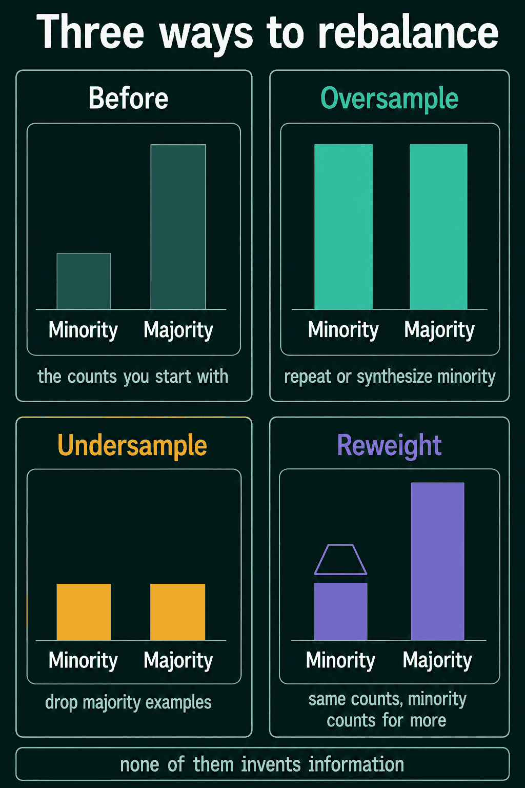
Better metrics show the problem, and rebalancing changes how the model learns. There are three common ways to do it, and none of them adds information the data does not already contain. They only change how much attention the model pays to each class.
The examples below use 1,000 labels, 980 legitimate (label 0) and 20 spam (label 1).
Reweighting
Reweighting leaves the data as it is and tells the loss to count each minority example as worth more. Nothing is copied or thrown away, which makes it the least destructive option. A common choice is to weight each class by the inverse of its frequency:
1import torch
2from torch import nn
3
4labels = torch.tensor([0] * 980 + [1] * 20)
5counts = torch.bincount(labels)
6weights = len(labels) / (2 * counts.float())
7print(counts)   # tensor([980,  20])
8print(weights)  # tensor([ 0.5102, 25.0000])
9
10loss_fn = nn.CrossEntropyLoss(weight=weights)
torch.bincount counts how many times each label appears. Dividing the total by twice each count gives every spam example 25 times the base weight and every legitimate one about half of it, so the two classes contribute about equally to the loss. The model sees each spam email once but pays 49 times more for getting one wrong.
Oversampling
Oversampling changes the counts by repeating minority examples until the classes match. Some methods create new synthetic examples instead of exact repeats. Here the 20 spam indices are drawn with replacement until there are 980 of them:
1import torch
2
3labels = torch.tensor([0] * 980 + [1] * 20)
4g = torch.Generator().manual_seed(0)
5spam_idx = (labels == 1).nonzero().squeeze(1)
6legit_idx = (labels == 0).nonzero().squeeze(1)
7
8extra = spam_idx[torch.randint(len(spam_idx), (len(legit_idx) - len(spam_idx),), generator=g)]
9oversampled = torch.cat([legit_idx, spam_idx, extra])
10print(torch.bincount(labels[oversampled]))  # tensor([980, 980])
The cost is that the same 20 spam emails now appear about 49 times each, so the model can memorize those exact messages instead of learning what spam looks like in general.
Undersampling
Undersampling goes the other way and drops majority examples until the classes match:
1import torch
2
3labels = torch.tensor([0] * 980 + [1] * 20)
4g = torch.Generator().manual_seed(0)
5spam_idx = (labels == 1).nonzero().squeeze(1)
6legit_idx = (labels == 0).nonzero().squeeze(1)
7
8keep = legit_idx[torch.randperm(len(legit_idx), generator=g)[:len(spam_idx)]]
9undersampled = torch.cat([keep, spam_idx])
10print(torch.bincount(labels[undersampled]))  # tensor([20, 20])
This keeps 40 of the 1,000 examples and throws away 960 real legitimate emails. Because of that loss, undersampling is often paired with reweighting rather than used alone, for example dropping some of the majority and weighting the rest.
| Method | What changes | Cost |
|---|---|---|
| Reweighting | the loss, not the data | the least destructive |
| Oversampling | minority examples repeated | the model can memorize them |
| Undersampling | majority examples dropped | real data thrown away |
When to rebalance
Check the label counts before training any classifier. If one class is a few percent of the data, plan to report precision, recall and F1 for it from the start. Try reweighting first, since it changes no data, and compare it with a model trained without rebalancing on the same validation set. Oversampling and undersampling are worth trying when reweighting does not move recall enough.
Common mistakes
- Reporting accuracy alone. On a 98/2 split, 98% is what a model that does nothing gets.
- Rebalancing the test set. The test set should keep the class mix the model will meet after deployment, or its scores say little about real use. Rebalance the training data only.
- Oversampling before splitting. Repeats of one spam email can land in both the training and the test set, so the model is tested on emails it trained on and the scores come out too high.
- Expecting rebalancing to fix too little data. Twenty spam emails repeated 49 times are still twenty spam emails. When recall stays low, labeling more minority examples usually helps more.
Related concepts
Class imbalance is one of several problems that can hide in a dataset, along with label errors, duplicates and test data that leaked into training. Labeling more minority examples brings back the questions of annotation and agreement between annotators. The post on train, validation and test splits covers why each split has its own job, which is why rebalancing belongs on the training split only.
QuiddityML teaches class imbalance as a concept in the NLP track's data unit. The exercises on it include ordering the lines of classification_metrics, spotting a recall that divides by the wrong total and an F1 written as a plain average, and writing the function from scratch (QuiddityML).