4 October 2026 · 11 min read

Precision, recall, and F1 score explained, with the confusion matrix

Precision, recall, and F1 score measure how well a classifier finds the cases you care about, which accuracy can hide. This post explains the confusion matrix they come from, what each metric tells you, how the decision threshold trades one for the other, and how to compute them in PyTorch.

Precision is the fraction of a classifier's "yes" answers that were correct, and recall is the fraction of the real "yes" cases it managed to find. The F1 score combines the two into one number, and the confusion matrix is the small table of counts that the three are calculated from. You meet them when a model has to pick out something rare, such as fraud, a disease, or spam, because on that kind of data the usual score, accuracy, can look excellent for a model that finds nothing.

Why accuracy is not enough

Accuracy is the fraction of predictions that are correct:

$$\text{accuracy} = \frac{\text{correct predictions}}{\text{total predictions}}$$

When the classes show up in similar numbers, accuracy is a reasonable score. When one class is rare, it stops telling you much.

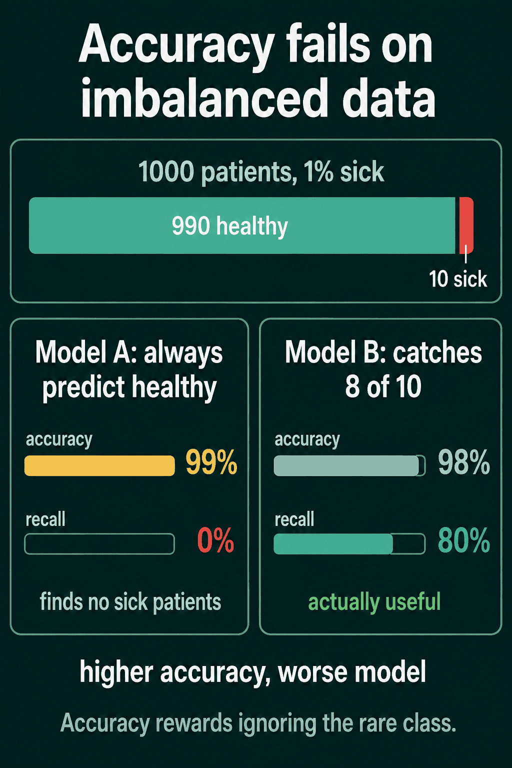
Take a test for a disease that affects 1% of people, run on 1000 patients: 990 are healthy and 10 are sick. Model A predicts "healthy" for each patient. It is right about the 990 healthy ones and wrong about the 10 sick ones, so its accuracy is 99%. Model B finds 8 of the 10 sick patients and raises 18 false alarms on healthy ones. It makes 20 mistakes, so its accuracy is 98%.

By accuracy, Model A wins. Model A has also not found a single sick patient, which is the reason the test exists. Accuracy counts a missed sick patient and a false alarm as the same kind of mistake, and with 990 healthy patients in the data, being right about them outweighs the 10 it gets wrong.

The four counts and the confusion matrix

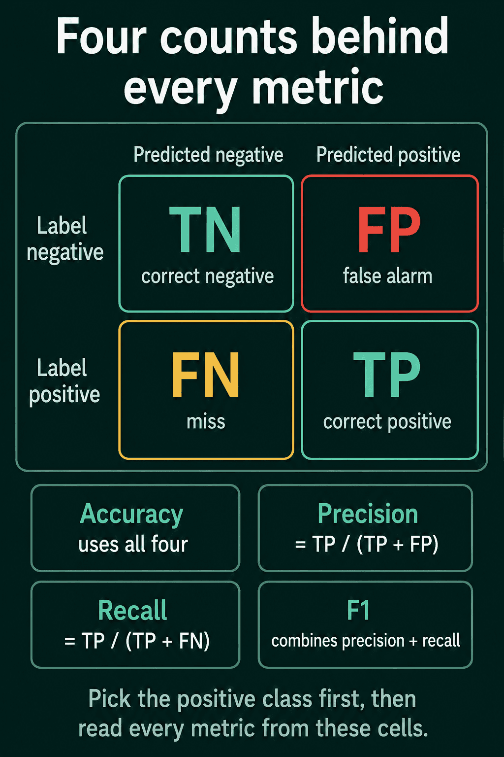
Start by choosing a positive class: the class you are trying to find. Here it is "sick". In a spam filter it would be "spam", in fraud detection "fraud". Which class you call positive is a choice, and the numbers below change if you flip it.

Each prediction then lands in one of four buckets:

True positive (TP): predicted positive, and the label is positive. A sick patient correctly flagged.
False positive (FP): predicted positive, but the label is negative. A false alarm.
False negative (FN): predicted negative, but the label is positive. A miss.
True negative (TN): predicted negative, and the label is negative. A healthy patient correctly cleared.

Laid out as a 2 by 2 table, these four counts are the confusion matrix. In this post the rows are the true label and the columns are the prediction, with the negative class first:

$$\begin{pmatrix} \text{TN} & \text{FP} \ \text{FN} & \text{TP} \end{pmatrix}$$

So the top row holds the patients who are actually healthy, and the bottom row the patients who are actually sick. The left column holds the patients the model called healthy, and the right column the ones it called sick. This is a common layout in Python libraries for labels 0 and 1, but some textbooks and tools transpose it and put TP in the top-left corner, so read the axis labels on a confusion matrix before reading a number off it.

For the two disease models:

Model A: TN = 990, FP = 0, FN = 10, TP = 0
Model B: TN = 972, FP = 18, FN = 2, TP = 8

Accuracy in these terms is the diagonal of the matrix divided by the total:

$$\text{accuracy} = \frac{\text{TP} + \text{TN}}{\text{TP} + \text{TN} + \text{FP} + \text{FN}}$$

What precision and recall measure

Precision and recall each look at one part of the matrix and ignore TN, the big pile of easy, correct negatives that inflated Model A's accuracy.

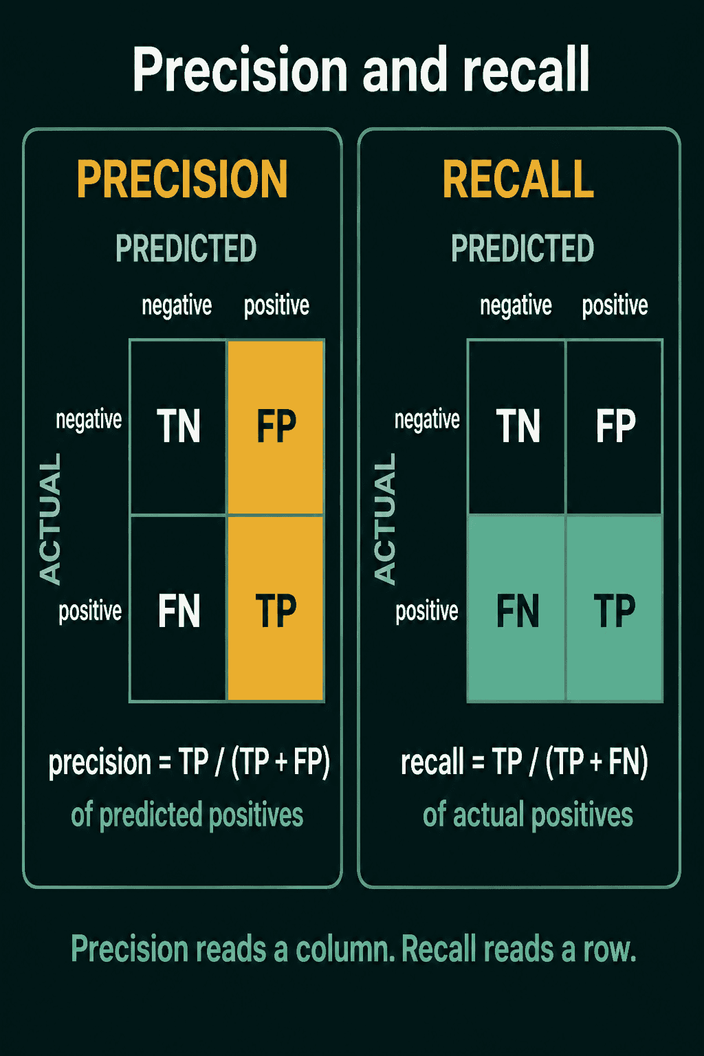
Precision asks: of the examples the model predicted positive, what fraction were really positive?

$$\text{precision} = \frac{\text{TP}}{\text{TP} + \text{FP}}$$

Recall asks: of the examples that really are positive, what fraction did the model find?

$$\text{recall} = \frac{\text{TP}}{\text{TP} + \text{FN}}$$

Each false alarm lowers precision, and each miss lowers recall.

For the disease models:

Model B: precision = 8 / (8 + 18) = 0.308, recall = 8 / (8 + 2) = 0.80
Model A: precision = 0 / (0 + 0), which is undefined because it made no positive predictions, and recall = 0 / (0 + 10) = 0

Recall shows at once that Model A is useless. Precision shows something about Model B that accuracy hid: when it flags a patient, it is right about 31% of the time, so roughly two out of three flagged patients are healthy.

A second example with round numbers: a spam filter flags 100 emails, and 90 of them are spam. Its precision is 90 / 100 = 0.90. If the inbox held 200 spam emails in total, the filter found 90 of 200, so its recall is 0.45 and it let 110 spam emails through. Precision needs no knowledge of how much spam exists. Recall needs no knowledge of how many legitimate emails exist.

In the matrix, precision reads down the predicted-positive column and recall reads across the actually-positive row.

Two copies of a 2 by 2 confusion matrix with actual class on the rows and predicted class on the columns, the left one shading the predicted-positive column (FP and TP) for precision and the right one shading the actual-positive row (FN and TP) for recall

Put side by side, the two disease models look very different once recall is next to accuracy:

1000 patients with 990 healthy and 10 sick, where Model A predicts healthy for each patient and gets 99% accuracy with 0% recall, while Model B catches 8 of 10 sick patients with 98% accuracy and 80% recall

The precision-recall tradeoff

The model outputs a probability $\hat{p}$ between 0 and 1, and you turn it into a decision with a threshold: predict positive when $\hat{p}$ is above the threshold, negative otherwise.

Moving the threshold moves precision and recall in opposite directions:

A high threshold, such as 0.8, makes the model say "positive" when it is very confident and not otherwise. It produces few false alarms, so precision goes up, and it misses more real positives, so recall goes down.
A low threshold, such as 0.2, makes the model say "positive" much more readily. It catches more real positives, so recall goes up, and it raises more false alarms, so precision goes down.

As a small example, take 10 patients, 4 sick and 6 healthy, scored by one model. At threshold 0.8 it flags 2 patients and both are sick: TP = 2, FP = 0, FN = 2, TN = 6, so precision is 1.00 and recall is 0.50. Lower the threshold to 0.2 and it flags 8 patients, which includes the 4 sick ones and 4 healthy ones: TP = 4, FP = 4, FN = 0, TN = 2, so precision drops to 0.50 and recall rises to 1.00. The model is the same in both cases, and the change comes from moving the line between "positive" and "negative".

Which side to favor depends on what each mistake costs:

Cancer screening: a missed cancer case is far worse than a follow-up test after a false alarm, so recall comes first.
Spam filter: a legitimate email sent to the spam folder is more damaging than one spam email reaching the inbox, so precision comes first.
Fraud detection: missed fraud costs money and false alarms annoy customers, so both need to stay reasonably high.

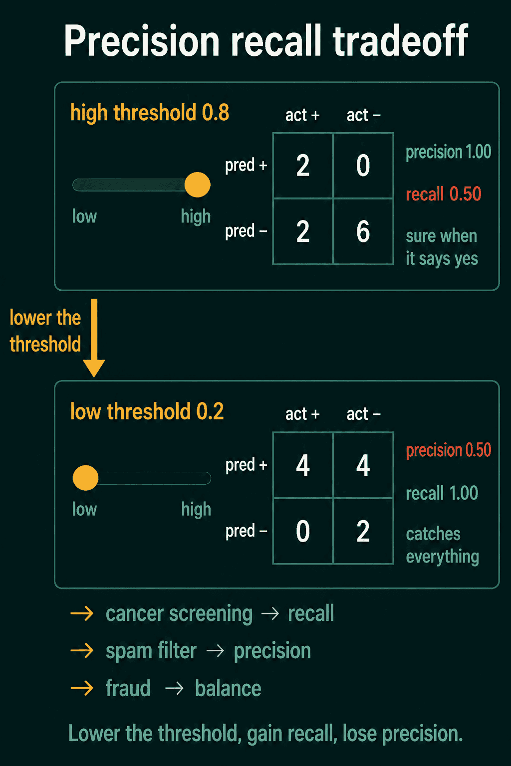
Two panels of the same 10 patients, where threshold 0.8 gives TP 2, FP 0, FN 2, TN 6 with precision 1.00 and recall 0.50, and threshold 0.2 gives TP 4, FP 4, FN 0, TN 2 with precision 0.50 and recall 1.00, plus cancer screening favoring recall, spam favoring precision, and fraud balancing both

This picture puts the prediction on the rows and the true label on the columns, the transpose of the layout used above.

The F1 score

Two numbers are awkward when you need to rank models or pick a threshold. The F1 score combines precision and recall into one number using their harmonic mean:

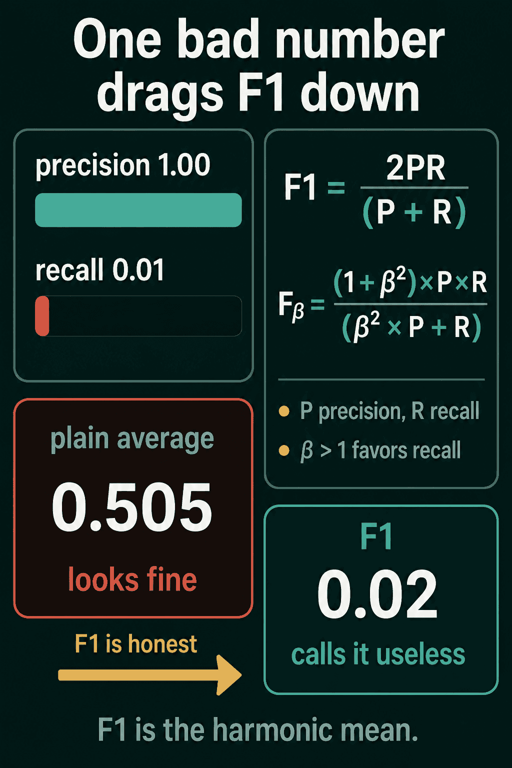
$$F_1 = \frac{2 \cdot \text{precision} \cdot \text{recall}}{\text{precision} + \text{recall}}$$

It is 1 when both are perfect, and it is pulled toward whichever of the two is lower.

A harmonic mean is used instead of a plain average because a plain average lets one good number hide a terrible one. With precision 1.0 and recall 0.01, a model that flags one patient correctly and misses 99 others, the plain average is 0.505, which reads like a middling model. F1 is $2 \cdot 1.0 \cdot 0.01 / (1.0 + 0.01) \approx 0.02$, which reads like the near-useless model it is. For Model B above, F1 is $2 \cdot 0.308 \cdot 0.80 / (0.308 + 0.80) \approx 0.444$.

F1 weights precision and recall equally. When one kind of mistake costs more, the F-beta score adds a weight $\beta$:

$$F_\beta = (1 + \beta^2) \cdot \frac{\text{precision} \cdot \text{recall}}{\beta^2 \cdot \text{precision} + \text{recall}}$$

With $\beta > 1$, recall counts for more, which suits problems where missing a positive is the worse mistake. With $\beta < 1$, precision counts for more.

Precision 1.00 and recall 0.01 give a plain average of 0.505 but an F1 of 0.02, shown next to the formulas for F1 and F-beta with P for precision and R for recall

Accuracy, precision, recall, and F1 are four different ratios of the same four cells, and each one exists because the others miss something:

The four cells TN, FP, FN, TP of a confusion matrix with label on the rows and prediction on the columns, with accuracy using the four cells, precision as TP over TP plus FP, recall as TP over TP plus FN, and F1 combining precision and recall

Computing them in PyTorch

The confusion matrix is a count of (label, prediction) pairs. For two classes, label * 2 + prediction turns each pair into a number from 0 to 3, and torch.bincount counts how often each number appears. Reshaped to 2 by 2, that is the matrix with rows as labels and columns as predictions. The script below rebuilds the two disease models:

1import torch
2 
3def confusion_matrix(preds, labels, num_classes=2):
4    # rows are the true label, columns are the prediction
5    idx = labels * num_classes + preds
6    counts = torch.bincount(idx, minlength=num_classes * num_classes)
7    return counts.reshape(num_classes, num_classes)
8 
9def metrics(cm):
10    tn, fp, fn, tp = cm.flatten().float()
11    accuracy = (tp + tn) / cm.sum()
12    precision = tp / (tp + fp)          # nan if the model makes no positive predictions
13    recall = tp / (tp + fn)
14    f1 = 2 * precision * recall / (precision + recall)
15    return accuracy.item(), precision.item(), recall.item(), f1.item()
16 
17# 1000 patients, the first 10 are sick (label 1)
18labels = torch.zeros(1000, dtype=torch.long)
19labels[:10] = 1
20 
21model_a = torch.zeros(1000, dtype=torch.long)   # predicts healthy for each patient
22model_b = torch.zeros(1000, dtype=torch.long)
23model_b[:8] = 1                                 # finds 8 of the 10 sick patients
24model_b[10:28] = 1                              # and raises 18 false alarms
25 
26for name, preds in [("A", model_a), ("B", model_b)]:
27    cm = confusion_matrix(preds, labels)
28    acc, p, r, f1 = metrics(cm)
29    print(f"model {name}: {cm.tolist()}  accuracy {acc:.3f}  precision {p:.3f}  recall {r:.3f}  F1 {f1:.3f}")

1model A: [[990, 0], [10, 0]]  accuracy 0.990  precision nan  recall 0.000  F1 nan
2model B: [[972, 18], [2, 8]]  accuracy 0.980  precision 0.308  recall 0.800  F1 0.444

Model A's precision comes out as nan with no error, because it made no positive predictions and 0.0 / 0.0 on a float tensor gives nan. That nan then spreads into F1.

To see the tradeoff, here are the same two functions applied to a model's probabilities at three thresholds. The data is synthetic: 1000 examples, 100 of them positive, with positives scoring higher on average:

1torch.manual_seed(0)
2labels = (torch.rand(1000) < 0.1).long()               # about 10% positives
3logits = torch.randn(1000) + 2.5 * labels - 1.0        # positives score higher on average
4probs = torch.sigmoid(logits)
5 
6for threshold in (0.2, 0.5, 0.8):
7    preds = (probs > threshold).long()
8    cm = confusion_matrix(preds, labels)
9    acc, p, r, f1 = metrics(cm)
10    print(f"threshold {threshold}: TP {cm[1, 1]:3d}  FP {cm[0, 1]:3d}  FN {cm[1, 0]:3d}  "
11          f"precision {p:.3f}  recall {r:.3f}  F1 {f1:.3f}")

1threshold 0.2: TP  99  FP 599  FN   1  precision 0.142  recall 0.990  F1 0.248
2threshold 0.5: TP  94  FP 152  FN   6  precision 0.382  recall 0.940  F1 0.543
3threshold 0.8: TP  55  FP   6  FN  45  precision 0.902  recall 0.550  F1 0.683

Going from 0.2 to 0.8, false alarms fall from 599 to 6 and precision climbs from 0.142 to 0.902, while misses rise from 1 to 45 and recall falls from 0.990 to 0.550. Of these three thresholds, F1 is highest at 0.8, but if missing a positive were the expensive mistake, 0.5 with recall 0.940 could be the better choice. If your numbers look wrong, check the matrix first: print it, and confirm which axis is the label and which class is positive.

More than two classes

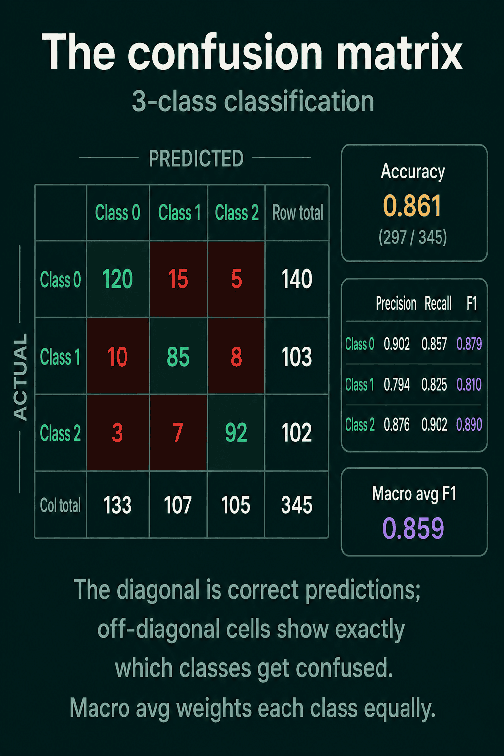
With three or more classes, the confusion matrix grows to one row and one column per class. The diagonal holds the correct predictions, and each off-diagonal cell counts how often one class was predicted as another. Precision, recall, and F1 are computed per class, treating that class as positive and the remaining classes as negative. For a class, precision divides its diagonal cell by its column total, and recall divides it by its row total. Averaging the per-class scores with equal weight gives the macro average, the "macro avg" row in many classification reports.

1import torch
2 
3cm = torch.tensor([[120, 15,  5],     # true class 0
4                   [ 10, 85,  8],     # true class 1
5                   [  3,  7, 92]])    # true class 2
6tp = cm.diag().float()
7precision = tp / cm.sum(dim=0)        # divide by each column: the examples predicted as that class
8recall = tp / cm.sum(dim=1)           # divide by each row: the examples that truly are that class
9f1 = 2 * precision * recall / (precision + recall)
10 
11print("accuracy ", round((tp.sum() / cm.sum()).item(), 3))
12print("precision", [round(x, 3) for x in precision.tolist()])
13print("recall   ", [round(x, 3) for x in recall.tolist()])
14print("F1       ", [round(x, 3) for x in f1.tolist()])
15print("macro F1 ", round(f1.mean().item(), 3))

1accuracy  0.861
2precision [0.902, 0.794, 0.876]
3recall    [0.857, 0.825, 0.902]
4F1        [0.879, 0.81, 0.889]
5macro F1  0.859

Accuracy is 0.861 and macro F1 is 0.859, and neither says where the 48 mistakes went, which the matrix shows directly: class 0 was predicted as class 1 fifteen times, and class 1 was predicted as class 0 ten times, so most of the confusion sits between those two classes. Two models can share the same aggregate score and fail in completely different ways, and the matrix shows which classes each one confuses.

A 3-class confusion matrix with actual class on the rows and predicted class on the columns, correct predictions on the diagonal, row and column totals, accuracy 0.861 (297 of 345), per-class precision, recall, and F1, and a macro average F1 of 0.859

The confusion_matrix function from the binary script handles this case too: pass num_classes=3.

When to use which, and common mistakes

Accuracy works when the classes are roughly balanced and both kinds of mistake cost about the same. When the positive class is rare, report precision and recall, and look at the confusion matrix before trusting any single score. Use F1 when you need one number to compare models and have no reason to favor precision or recall, and F-beta when you do. Set the threshold by the metric that matches the cost of each mistake.

Reporting accuracy on imbalanced data. A model that predicts the majority class for each example scores 99% on data with 1% positives and finds nothing.
Reading the matrix the wrong way round. Rows as labels and columns as predictions is a common layout, not a universal one. A transposed matrix swaps FP and FN, which swaps precision and recall.
Forgetting which class is positive. Calling the other class positive turns false positives into false negatives and the reverse, so precision, recall, and F1 come out different.

Precision, recall, and F1 are measured at one threshold. The ROC curve and AUC post looks at a model across many thresholds instead. When the dataset is small, the cross-validation post shows how to get these numbers from more than one split.

QuiddityML teaches accuracy, precision and recall, the precision-recall tradeoff, F1, and the confusion matrix as their own concepts in the ML Foundation track, and the exercises on them include working out a spam filter's precision and recall by hand, spotting a recall function that counts false negatives with the wrong condition, and writing precision, recall, and F1 from scratch.