By Sagi Shaier · 9 October 2026 · 5 min read

The condition number explained: why some problems are numerically unstable

How to compute the condition number of a matrix from its eigenvalues, what the Rayleigh quotient says about the largest and smallest eigenvalue, and two PyTorch experiments that show a large condition number amplifying small errors and slowing gradient descent.

The condition number of a matrix is the ratio of its largest eigenvalue size to its smallest, and it measures how unevenly the matrix stretches different directions. A condition number near 1 means every direction is treated about the same, and a large one means a linear system built on that matrix amplifies small errors and gradient descent on a loss with that curvature moves slowly.

The Rayleigh quotient

An eigenvalue $\lambda$ of a matrix $A$ is the factor by which $A$ scales one of its special directions, an eigenvector $\mathbf{v}$, so $A\mathbf{v} = \lambda\mathbf{v}$. For a symmetric matrix (one equal to its own transpose), every eigenvalue is a real number.

For a symmetric matrix, the eigenvalues also answer an optimization question: how large or small can $\mathbf{x}^\top A \mathbf{x}$ get when $\mathbf{x}$ points in any direction? The expression that asks it, for any nonzero $\mathbf{x}$, is the Rayleigh quotient:

$$R(\mathbf{x}) = \frac{\mathbf{x}^\top A \mathbf{x}}{\mathbf{x}^\top \mathbf{x}}$$

Dividing by $\mathbf{x}^\top\mathbf{x}$, the squared length of $\mathbf{x}$, removes the effect of length, so $R(\mathbf{x})$ depends only on the direction of $\mathbf{x}$. Its values always stay between the smallest and the largest eigenvalue:

$$\lambda_{\min} \leq R(\mathbf{x}) \leq \lambda_{\max}$$

and it reaches each end exactly when $\mathbf{x}$ is the matching eigenvector.

Take the matrix with rows $(4, 0)$ and $(0, 1)$, whose eigenvalues are 4 and 1. Sweeping a unit vector $\mathbf{x}$ around from 0 to 180 degrees, $R(\mathbf{x})$ starts at 4 along the first axis, falls to 1 at 90 degrees along the second axis, and climbs back to 4.

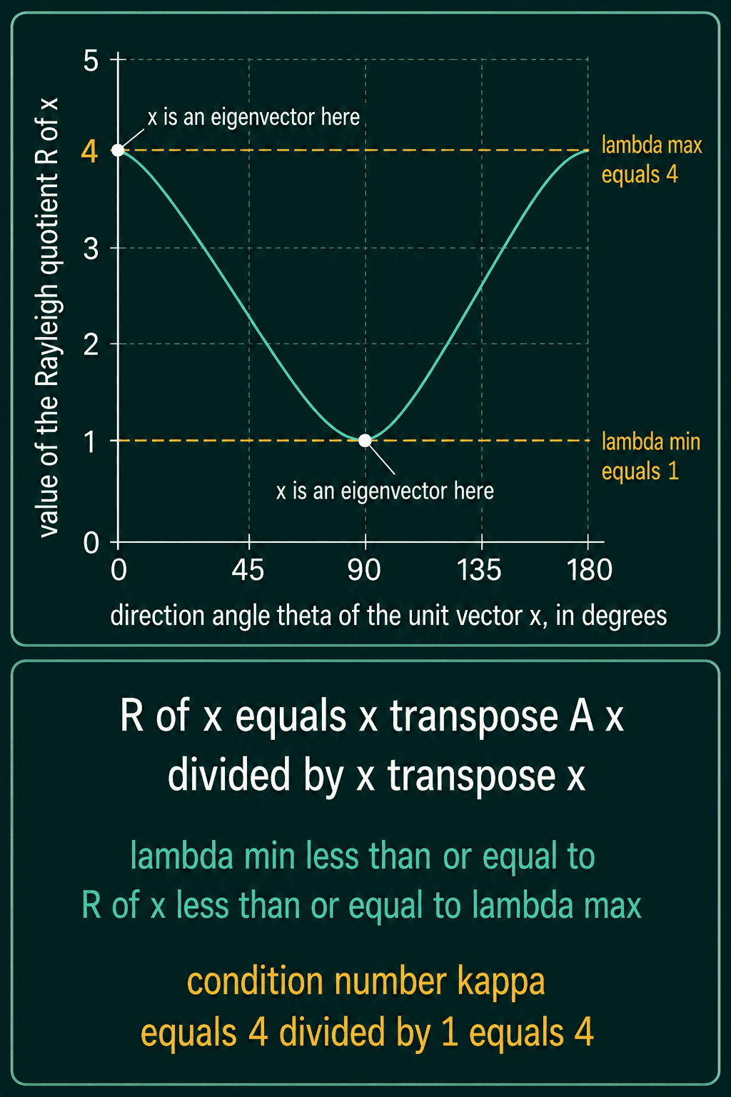
The Rayleigh quotient of the matrix with eigenvalues 4 and 1, plotted against the angle of a unit vector x from 0 to 180 degrees: it starts at lambda max = 4, drops to lambda min = 1 at 90 degrees, and returns to 4, touching each end where x is an eigenvector. The condition number is 4 divided by 1 = 4

This is how PCA finds the direction of greatest variance in a dataset: it is the eigenvector of the covariance matrix with the largest eigenvalue, because that direction maximizes the Rayleigh quotient.

The condition number

The ratio between the largest and smallest eigenvalue sizes is the condition number, written $\kappa$ (kappa):

$$\kappa(A) = \frac{\max_i |\lambda_i|}{\min_i |\lambda_i|}$$

$|\lambda|$ is the absolute value of an eigenvalue. The absolute values handle indefinite matrices, which have a mix of positive and negative eigenvalues: the comparison is between the largest and smallest sizes, not the most positive and most negative values. That also means the condition number is never less than 1. For a matrix whose eigenvalues are all zero or positive, the absolute values change nothing. For the matrix above, $\kappa = 4 / 1 = 4$.

For a general matrix that is not symmetric, the condition number uses singular values instead of eigenvalues, which are never negative by construction.

What a large condition number does

A condition number close to 1 means the matrix stretches every direction about equally. A large condition number means some directions get stretched far more than others, and that imbalance causes two practical problems:

Solving a linear system $A\mathbf{x} = \mathbf{b}$ becomes unstable. A tiny change in $\mathbf{b}$, such as a rounding error or a little measurement noise, can produce a large change in the solution $\mathbf{x}$.
Gradient descent slows down. When the curvature of a loss differs a lot between directions, the loss surface is a long narrow valley. A step size small enough to stay stable along the steep direction makes very slow progress along the shallow one.

Experiments in PyTorch

The Rayleigh quotient and the condition number for the matrix with eigenvalues 4 and 1:

1import math
2import torch
3 
4A = torch.tensor([[4.0, 0.0],
5                  [0.0, 1.0]])
6 
7def rayleigh(A, x):
8    return (x @ A @ x) / (x @ x)
9 
10for deg in (0, 45, 90, 135, 180):
11    t = math.radians(deg)
12    x = torch.tensor([math.cos(t), math.sin(t)])
13    print(deg, round(rayleigh(A, x).item(), 3))
14 
15vals = torch.linalg.eigvalsh(A)
16print(vals.abs().max() / vals.abs().min(), torch.linalg.cond(A))

10 4.0
245 2.5
390 1.0
4135 2.5
5180 4.0
6tensor(4.) tensor(4.)

torch.linalg.cond computes the condition number directly. A system whose matrix has two nearly identical rows is badly conditioned, and changing $\mathbf{b}$ by 0.001 moves the solution a long way:

1import torch
2 
3A = torch.tensor([[1.0, 1.0],
4                  [1.0, 1.001]], dtype=torch.float64)
5print(torch.linalg.cond(A))
6 
7b = torch.tensor([2.0, 2.001], dtype=torch.float64)
8print(torch.linalg.solve(A, b))
9b2 = torch.tensor([2.0, 2.002], dtype=torch.float64)   # change b by 0.001
10print(torch.linalg.solve(A, b2))

1tensor(4002.0008, dtype=torch.float64)
2tensor([1., 1.], dtype=torch.float64)
3tensor([0., 2.], dtype=torch.float64)

The condition number is about 4,000, and a change of 0.001 in one entry of $\mathbf{b}$ moves the solution from $(1, 1)$ to $(0, 2)$.

Gradient descent on $f(\mathbf{x}) = \frac{1}{2}\mathbf{x}^\top A \mathbf{x}$, whose curvature is set by $A$ and whose gradient is $A\mathbf{x}$, with a well-conditioned and an ill-conditioned $A$:

1import torch
2 
3def steps_to_converge(A, lr, tol=1e-6):
4    """Gradient descent on f(x) = 0.5 x^T A x, starting at (1, 1)."""
5    x = torch.tensor([1.0, 1.0], dtype=torch.float64)
6    for step in range(1, 100_000):
7        x = x - lr * (A @ x)           # the gradient of f is A x
8        if x.norm() < tol:
9            return step
10 
11well = torch.diag(torch.tensor([1.0, 1.0], dtype=torch.float64))    # condition number 1
12ill = torch.diag(torch.tensor([100.0, 1.0], dtype=torch.float64))   # condition number 100
13print(steps_to_converge(well, lr=1.0 / 1.0))
14print(steps_to_converge(ill, lr=1.0 / 100.0))

11
21375

Both runs use the largest step size that keeps the steep direction stable, 1 divided by the largest eigenvalue. With condition number 1, one step lands on the minimum. With condition number 100, the same step size moves only 1% of the way along the shallow direction each step, and it takes 1,375 steps. If a solve or a fit gives results that jump around with small changes to the data, torch.linalg.cond on the matrix involved is a quick first check.

Common mistakes

Dividing the most positive eigenvalue by the most negative. The condition number compares sizes, so it uses absolute values and is never below 1.
Using eigenvalues for a matrix that is not symmetric. For a general matrix, the condition number comes from singular values.
Reading a small determinant as a large condition number. Scaling a whole matrix by 0.001 shrinks its determinant and leaves its condition number unchanged.
Building $A^\top A$ when solving least squares. That squares the condition number, which is why factorizations like QR avoid forming it.

Eigenvalues and eigenvectors are covered in eigenvalues and eigenvectors explained, and the QR factorization that avoids squaring the condition number is in positive definite matrices, Cholesky and QR. SVD gives the singular values used for the condition number of a general matrix.

QuiddityML teaches the Rayleigh quotient and the condition number as one concept in the linear algebra part of the Math track, and the exercises include filling in the condition number formula, ordering the lines of a condition_number function, and writing it from scratch.