By Sagi Shaier · 9 October 2026 · 6 min read

Eigenvalues and eigenvectors explained

How to find the eigenvalues and eigenvectors of a matrix, how they relate to its determinant and trace, how a change of basis rewrites a vector or a matrix, and how eigendecomposition turns a matrix into per-axis scaling, with PyTorch code throughout.

An eigenvector of a matrix is a direction the matrix only stretches, shrinks, or flips, without turning it, and the eigenvalue is the factor it gets scaled by. PCA finds the directions of greatest spread in a dataset as the eigenvectors of its covariance matrix, and an eigenvalue near zero shows a direction the matrix nearly collapses, which is how singular matrices and lost rank show up.

What an eigenvector is

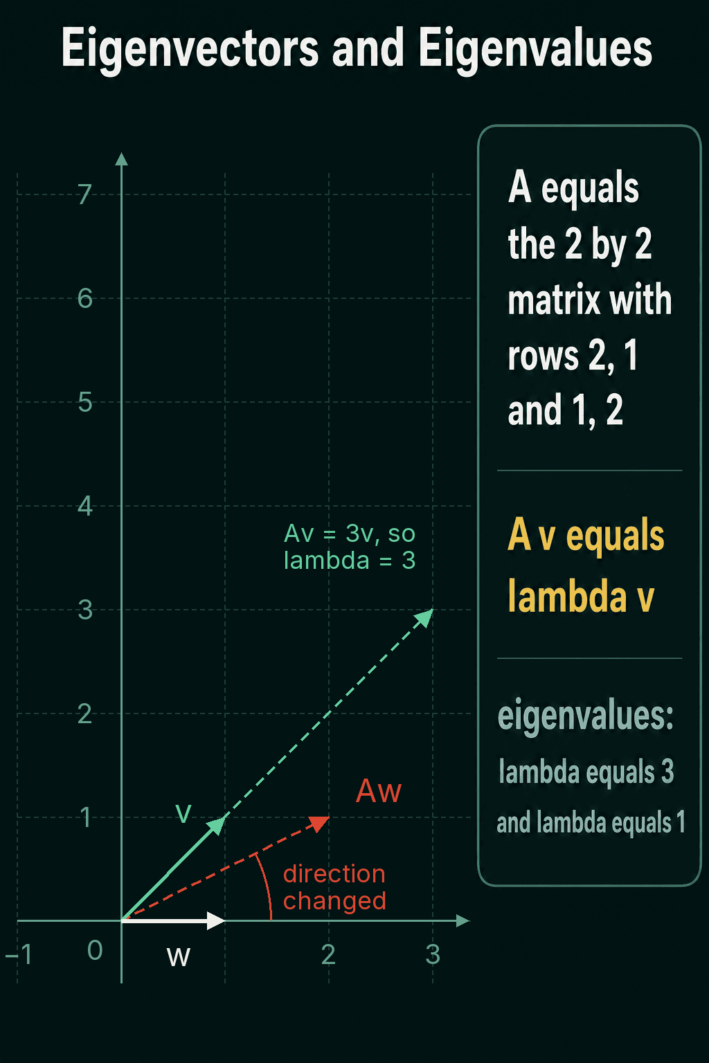
A matrix $A$ transforms vectors: multiplying a vector by $A$ can stretch it, rotate it, or shear it. Most vectors come out pointing in a new direction. A few special directions come out pointing the same way as they went in, only longer, shorter, or flipped. A vector $\mathbf{v}$ in one of those directions is an eigenvector of $A$, and the number $\lambda$ (lambda) it gets scaled by is its eigenvalue:

$$A\mathbf{v} = \lambda\mathbf{v}$$

The equation says that applying the whole matrix $A$ to $\mathbf{v}$ does the same thing as multiplying $\mathbf{v}$ by the single number $\lambda$.

Take the matrix $A$ with rows $(2, 1)$ and $(1, 2)$. For $\mathbf{v} = (1, 1)$:

$$A\mathbf{v} = (2 + 1, 1 + 2) = (3, 3) = 3\mathbf{v}$$

so $\mathbf{v}$ is an eigenvector with eigenvalue 3. For $\mathbf{w} = (1, 0)$, $A\mathbf{w} = (2, 1)$, which points in a different direction, so $\mathbf{w}$ is not an eigenvector. The other eigenvalue of this matrix is 1, with eigenvector $(-1, 1)$.

The matrix A with rows (2, 1) and (1, 2): v = (1, 1) maps to Av = (3, 3), the same direction scaled by 3, while w = (1, 0) maps to Aw = (2, 1) and changes direction. The eigenvalues are 3 and 1

Finding eigenvalues

Move everything in the definition to one side: $A\mathbf{v} - \lambda\mathbf{v} = \mathbf{0}$, which is $(A - \lambda I)\mathbf{v} = \mathbf{0}$, where $I$ is the identity matrix. For a nonzero $\mathbf{v}$ to solve this, the matrix $A - \lambda I$ has to be singular, meaning it has no inverse, which happens exactly when its determinant is 0:

$$\det(A - \lambda I) = 0$$

This is the characteristic equation. For the matrix above it is $(2 - \lambda)^2 - 1 = 0$, which gives $\lambda = 3$ and $\lambda = 1$. For anything larger than a small matrix, torch.linalg.eig (or torch.linalg.eigh for symmetric matrices) does the work.

Two summaries of a matrix come straight from its eigenvalues:

The determinant is the product of the eigenvalues: $3 \times 1 = 3$, and $\det(A) = 2 \times 2 - 1 \times 1 = 3$. If any eigenvalue is 0, the determinant is 0 and the matrix is singular.
The trace, the sum of the diagonal entries, is the sum of the eigenvalues: $3 + 1 = 4$, and $2 + 2 = 4$.

Change of basis

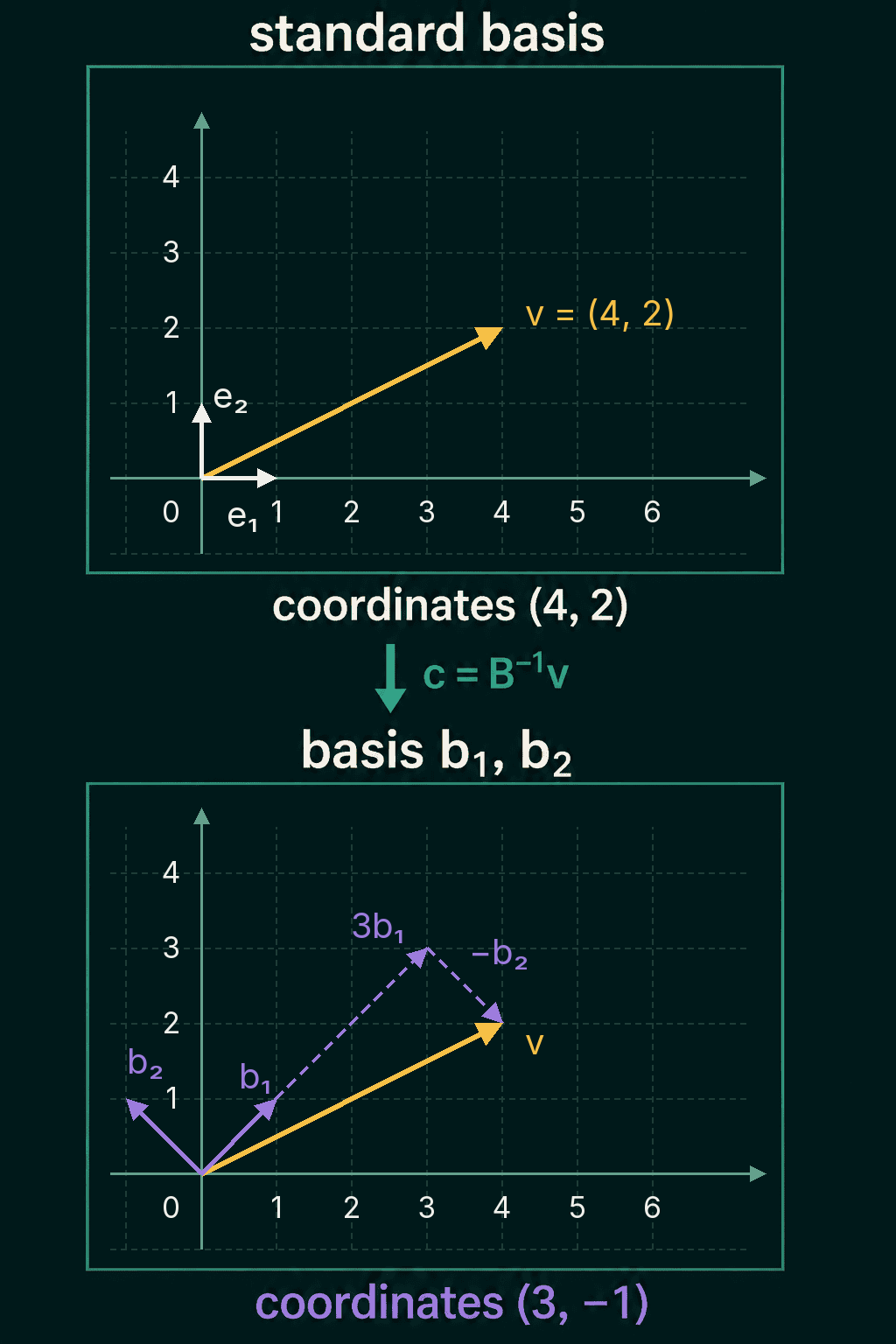
The numbers in a vector like $(4, 2)$ are coordinates measured against the standard basis $(1, 0)$ and $(0, 1)$: 4 steps along the first, 2 along the second. Any other basis, a set of independent vectors that can build every vector in the space, can play the same role, and the same vector then gets different coordinates.

Pick a new basis $\mathbf{b}_1, \mathbf{b}_2$ and stack the two vectors as the columns of a matrix $B$. The coordinates $\mathbf{c} = (c_1, c_2)$ of $\mathbf{v}$ in the new basis satisfy $\mathbf{v} = c_1\mathbf{b}_1 + c_2\mathbf{b}_2$, which is the system of equations

$$B\mathbf{c} = \mathbf{v} \quad\Longrightarrow\quad \mathbf{c} = B^{-1}\mathbf{v}$$

With $\mathbf{b}_1 = (1, 1)$ and $\mathbf{b}_2 = (-1, 1)$, the vector $(4, 2)$ has coordinates $(3, -1)$, since $3(1, 1) - 1(-1, 1) = (4, 2)$.

The vector (4, 2) drawn twice: in the standard basis with coordinates (4, 2), and in the basis b1 = (1, 1), b2 = (-1, 1), where it is 3 b1 minus b2, so its coordinates are (3, -1)

A matrix can be rewritten in a new basis too. If $A$ is a transformation written in standard coordinates, the same transformation written in the $B$ basis is

$$A' = B^{-1}AB$$

Read it right to left: $B$ turns $B$-basis coordinates into standard ones, $A$ transforms them, and $B^{-1}$ turns the result back into $B$-basis coordinates. Some bases make a transformation look much simpler than others, and the eigenvectors of a matrix are the basis that makes it simplest.

Eigendecomposition

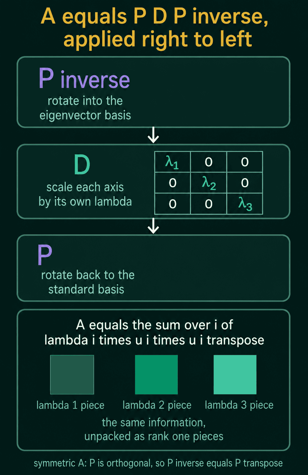
If a matrix $A$ has enough independent eigenvectors, stack them as the columns of a matrix $P$, and put the matching eigenvalues on the diagonal of a matrix $D$, with zeros everywhere else. Then:

$$A = PDP^{-1}$$

This is eigendecomposition, and a matrix that can be written this way is diagonalizable. It is the change of basis above with $P$ in the role of $B$. Reading right to left: $P^{-1}$ changes coordinates into the eigenvector basis, $D$ scales each axis by its own eigenvalue, and $P$ changes back to standard coordinates.

A = P D P inverse read right to left: P inverse moves into the eigenvector basis, D scales each axis by its own eigenvalue, P moves back to the standard basis, and the same matrix written as a sum of eigenvalue-weighted pieces

One payoff is matrix powers. Applying $A$ $k$ times is expensive to compute directly, and with the decomposition

$$A^k = PD^kP^{-1}$$

where $D^k$ only raises each diagonal entry to the power $k$. Directions with eigenvalues larger than 1 in size grow under repeated application, and directions with eigenvalues smaller than 1 in size shrink.

Not every matrix is diagonalizable, since some do not have enough independent eigenvectors to fill $P$.

Symmetric matrices

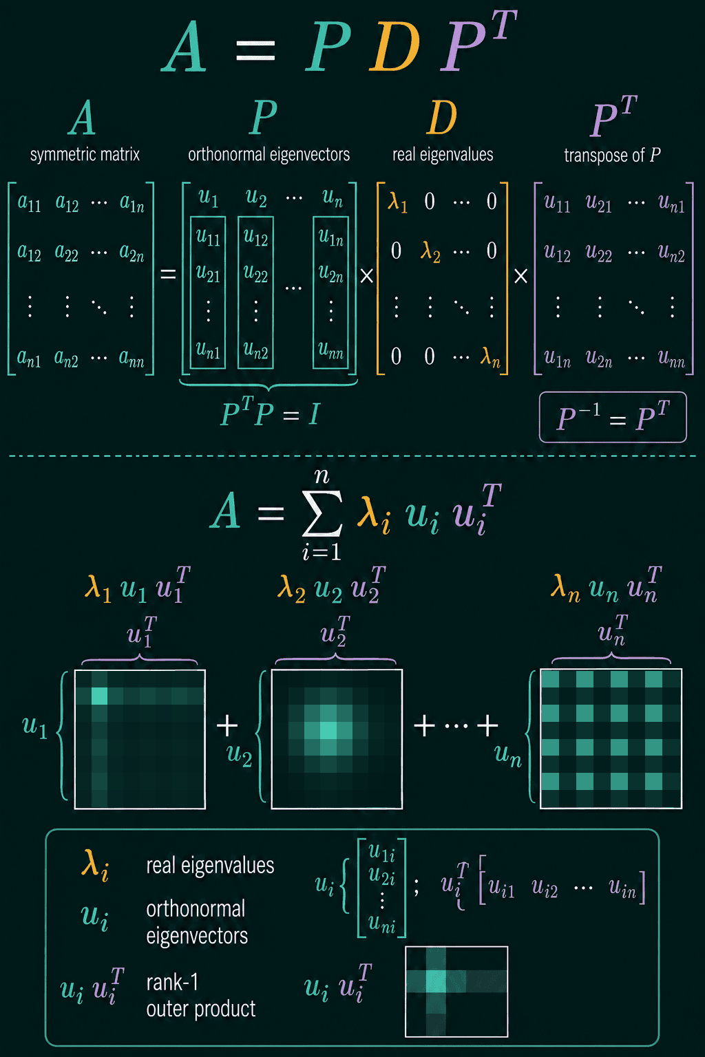
A symmetric matrix equals its own transpose, $A = A^\top$. Every symmetric matrix is diagonalizable, its eigenvalues are real numbers, and its eigenvectors can be chosen to have length 1 and sit at right angles to each other (orthonormal). That makes $P$ an orthogonal matrix, whose inverse is its transpose, so:

$$A = PDP^\top$$

Covariance matrices are symmetric, which is why PCA can use their eigendecomposition. The same decomposition can be written one eigenvector at a time, with $\mathbf{u}_i$ the $i$-th column of $P$:

$$A = \sum_i \lambda_i \mathbf{u}_i \mathbf{u}_i^\top$$

Each $\mathbf{u}_i \mathbf{u}_i^\top$ is an outer product, a matrix built from one vector, scaled by its eigenvalue. Keeping only the terms with the largest eigenvalues gives a smaller approximation of $A$.

A symmetric matrix written as P D P transpose, with orthonormal eigenvectors in P and real eigenvalues in D, and the same matrix as a sum of eigenvalue-weighted outer products, each a rank-1 matrix

Eigenvalues in PyTorch

1import torch
2 
3A = torch.tensor([[2.0, 1.0],
4                  [1.0, 2.0]])
5v = torch.tensor([1.0, 1.0])
6w = torch.tensor([1.0, 0.0])
7print(A @ v, A @ w)                    # v only gets scaled, w changes direction
8 
9vals, vecs = torch.linalg.eigh(A)      # for symmetric matrices
10print(vals)
11print(vecs)
12print(torch.linalg.det(A), vals.prod())   # determinant = product of eigenvalues
13print(torch.trace(A), vals.sum())         # trace = sum of eigenvalues

1tensor([3., 3.]) tensor([2., 1.])
2tensor([1., 3.])
3tensor([[-0.7071,  0.7071],
4        [ 0.7071,  0.7071]])
5tensor(3.) tensor(3.)
6tensor(4.) tensor(4.)

torch.linalg.eigh returns the eigenvalues smallest first, and the eigenvectors as unit-length columns in the same order: $(-0.7071, 0.7071)$ is $(-1, 1)$ scaled to length 1, and $(0.7071, 0.7071)$ is $(1, 1)$ scaled the same way. For a matrix that is not symmetric, use torch.linalg.eig, which returns complex numbers.

Change of basis and eigendecomposition:

1import torch
2 
3# change of basis: coordinates of v in the basis b1 = (1, 1), b2 = (-1, 1)
4B = torch.tensor([[1.0, -1.0],
5                  [1.0,  1.0]])        # b1 and b2 as columns
6v = torch.tensor([4.0, 2.0])
7c = torch.linalg.solve(B, v)
8print(c, B @ c)
9 
10# eigendecomposition A = P D P^T and a matrix power through it
11A = torch.tensor([[2.0, 1.0],
12                  [1.0, 2.0]])
13vals, P = torch.linalg.eigh(A)
14D = torch.diag(vals)
15print(P @ D @ P.T)
16print(P @ torch.diag(vals ** 5) @ P.T)
17print(torch.linalg.matrix_power(A, 5))

1tensor([ 3., -1.]) tensor([4., 2.])
2tensor([[2.0000, 1.0000],
3        [1.0000, 2.0000]])
4tensor([[122., 121.],
5        [121., 122.]])
6tensor([[122., 121.],
7        [121., 122.]])

torch.linalg.solve(B, v) finds the coordinates without forming $B^{-1}$. Raising the two eigenvalues to the 5th power and multiplying back gives the same $A^5$ as multiplying $A$ by itself five times. If a reconstruction $P D P^{-1}$ does not match $A$, check whether the matrix is symmetric: $P^\top$ replaces $P^{-1}$ only in that case.

Common mistakes

Expecting a unique eigenvector. Any nonzero multiple of an eigenvector is also an eigenvector, so $(1, 1)$, $(2, 2)$ and $(-0.7071, -0.7071)$ all describe the same direction.
Using eigh on a matrix that is not symmetric. It reads only one triangle of the matrix and returns wrong answers without an error.
Writing $P^\top$ instead of $P^{-1}$ for a general matrix. That shortcut holds only when $P$ is orthogonal, as it is for symmetric matrices.
Mixing up determinant and trace. The determinant multiplies the eigenvalues and the trace adds them.

Orthogonal matrices, whose inverse is their transpose, are covered in orthogonality explained. The determinant and trace themselves are in determinant, inverse and trace explained. Positive definite matrices are the symmetric matrices whose eigenvalues are all positive.

QuiddityML teaches eigenvectors, change of basis and eigendecomposition as three concepts in the linear algebra part of the Math track, and the exercises include tracing whether a vector is an eigenvector of a matrix, ordering the steps that compute $A^k$ through the decomposition, and writing reconstruct from scratch.