By Sagi Shaier · 9 October 2026 · 6 min read
Positive definite matrices explained, with the Cholesky and QR factorizations
How to test whether a matrix is positive definite, semi-definite, negative definite or indefinite, why every covariance matrix passes the semi-definite test, and when to use the QR and Cholesky factorizations, with PyTorch code for each.
A symmetric matrix is positive definite when all of its eigenvalues are greater than zero, and positive semi-definite when they are all zero or greater. Every covariance matrix is positive semi-definite, the curvature test that separates a minimum from a maximum or a saddle point uses the same categories, and the Cholesky factorization, used to sample correlated Gaussian noise, needs a positive definite matrix to work.
The eigenvalue test
A symmetric matrix equals its own transpose ($A = A^\top$), and its eigenvalues, the factors $\lambda$ by which it scales its special directions ($A\mathbf{v} = \lambda\mathbf{v}$), are all real numbers. The signs of those eigenvalues sort symmetric matrices into five groups:
| Category | Eigenvalues |
|---|---|
| positive definite | all $> 0$ |
| positive semi-definite | all $\geq 0$ |
| negative definite | all $< 0$ |
| negative semi-definite | all $\leq 0$ |
| indefinite | some positive, some negative |
The quadratic form test
There is an equivalent test that needs no eigenvalues. For a vector $\mathbf{x}$, the number $\mathbf{x}^\top A \mathbf{x}$ is called a quadratic form. $A$ is positive semi-definite exactly when
$$\mathbf{x}^\top A \mathbf{x} \geq 0$$
for every vector $\mathbf{x}$, and positive definite when $\mathbf{x}^\top A \mathbf{x} > 0$ for every nonzero $\mathbf{x}$. Negative definite flips the sign, $\mathbf{x}^\top A \mathbf{x} < 0$ for every nonzero $\mathbf{x}$. For an indefinite matrix, $\mathbf{x}^\top A \mathbf{x}$ comes out positive for some $\mathbf{x}$ and negative for others.
Plotting $\mathbf{x}^\top A \mathbf{x}$ over 2D inputs shows the three shapes: a bowl that only goes up from the origin, an upside-down bowl that only goes down, and a saddle that goes up in some directions and down in others.
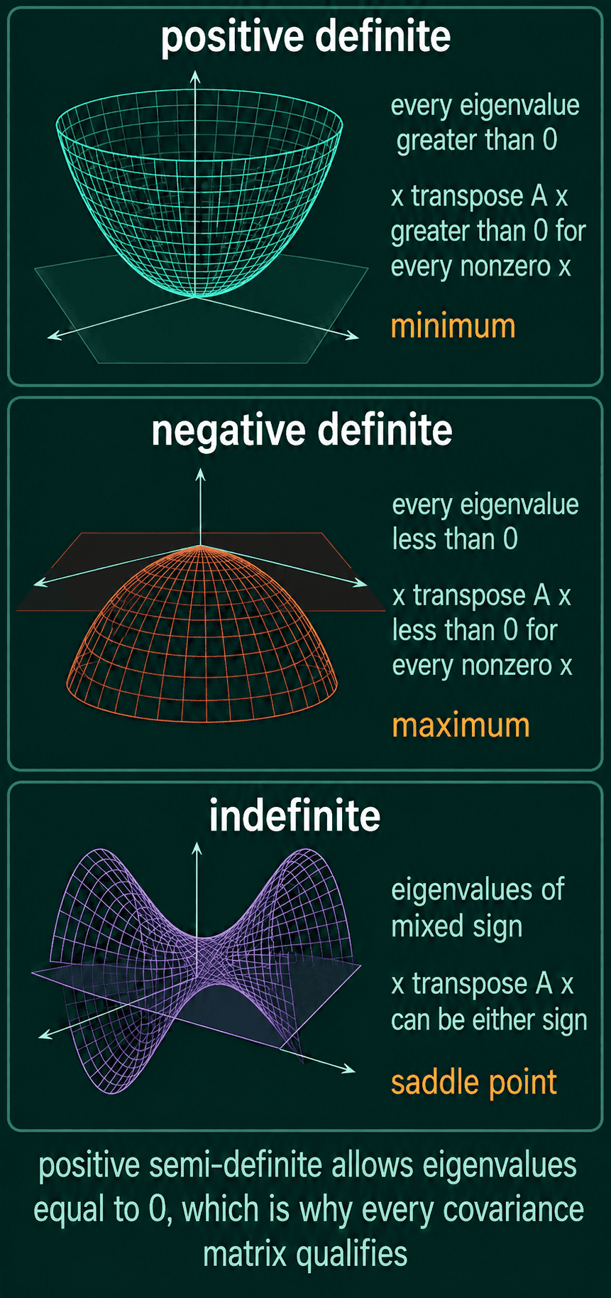
When the matrix is the Hessian of a function (the matrix of its second derivatives) at a point where the slope is zero, the categories classify that point: positive definite is a minimum, negative definite is a maximum, and indefinite is a saddle point.
Two quick checks rule a matrix out early. A positive definite matrix has $\det(A) > 0$ and every diagonal entry positive. Both are necessary, and neither one is enough on its own to prove a matrix is positive definite.
Why every covariance matrix is positive semi-definite
For a covariance matrix $C$ and a direction $\mathbf{x}$ of length 1, $\mathbf{x}^\top C \mathbf{x}$ is the variance of the data projected onto that direction. Variance cannot be negative, so $\mathbf{x}^\top C \mathbf{x} \geq 0$ for every direction, which is the positive semi-definite test. A negative eigenvalue would mean a direction with negative variance.
The same condition decides which functions can be kernels in kernel methods: a function qualifies as a kernel only if the matrix of its values over any set of points is positive semi-definite.
Checking the categories in PyTorch
torch.linalg.eigvalsh returns the real eigenvalues of a symmetric matrix, sorted smallest to largest. torch.linalg.eig works on any square matrix and returns complex numbers, even when every imaginary part is zero, which makes comparing against 0 awkward. The h stands for Hermitian, the complex-number name for symmetric.
1import torch
2
3def classify(A):
4    vals = torch.linalg.eigvalsh(A)    # real eigenvalues, smallest first
5    if (vals > 0).all():  return 'positive definite'
6    if (vals >= 0).all(): return 'positive semi-definite'
7    if (vals < 0).all():  return 'negative definite'
8    if (vals <= 0).all(): return 'negative semi-definite'
9    return 'indefinite'
10
11for A in ([[2.0, 1.0], [1.0, 2.0]],
12          [[1.0, 1.0], [1.0, 1.0]],
13          [[-3.0, 0.0], [0.0, -1.0]],
14          [[1.0, 0.0], [0.0, -1.0]]):
15    A = torch.tensor(A)
16    print(torch.linalg.eigvalsh(A), classify(A))
17
18# a covariance matrix is positive semi-definite
19torch.manual_seed(0)
20X = torch.randn(200, 3)
21C = torch.cov(X.T)
22print(torch.linalg.eigvalsh(C))1tensor([1., 3.]) positive definite
2tensor([0., 2.]) positive semi-definite
3tensor([-3., -1.]) negative definite
4tensor([-1., 1.]) indefinite
5tensor([0.8795, 1.0839, 1.1318])On real data, an eigenvalue that should be exactly 0 can come out as a tiny negative number like $-10^{-7}$ from rounding, so a practical check compares against a small negative tolerance such as vals >= -1e-6 instead of vals >= 0.
QR decomposition
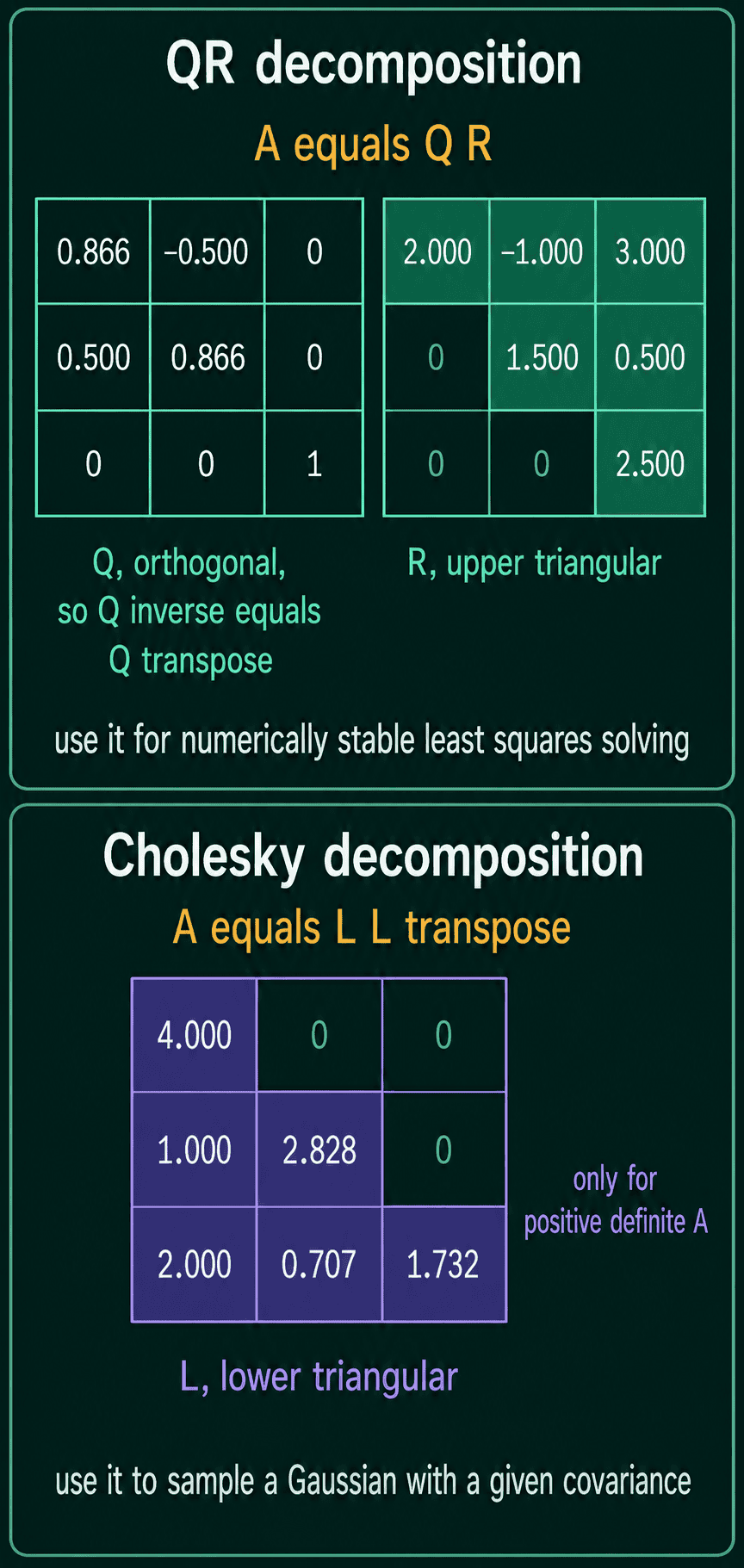
QR decomposition writes any matrix as $A = QR$, where $Q$ has orthonormal columns (each of length 1, all at right angles to each other) and $R$ is upper triangular (zeros everywhere below the diagonal). When $A$ is square, $Q$ is an orthogonal matrix.
Its main use is solving least squares problems, finding the $\mathbf{x}$ that brings $A\mathbf{x}$ closest to a target $\mathbf{b}$ when no exact solution exists. The textbook route goes through the normal equations $A^\top A\mathbf{x} = A^\top\mathbf{b}$. Substitute $A = QR$ and use $Q^\top Q = I$:
$$R^\top Q^\top QR\mathbf{x} = R^\top Q^\top\mathbf{b}$$
$$R^\top R\mathbf{x} = R^\top Q^\top\mathbf{b}$$
$$R\mathbf{x} = Q^\top\mathbf{b}$$
$Q^\top\mathbf{b}$ costs one matrix product, and because $R$ is upper triangular the last system solves from the bottom row up, one unknown at a time, called back-substitution. The matrix $A^\top A$ never gets built. Building it squares the condition number of the problem, a measure of how much small rounding errors get amplified, so the QR route stays more accurate.
Cholesky decomposition
Cholesky decomposition applies only to positive definite matrices. It writes $A = LL^\top$, where $L$ is lower triangular (zeros everywhere above the diagonal). It works as a square root for matrices: a positive definite matrix has one in the same way a positive number does.
Its common use in machine learning is sampling from a multivariate Gaussian with a chosen covariance matrix $C$. Start with independent standard-normal samples $\mathbf{z}$, compute $L$ from $C = LL^\top$, and multiply: $L\mathbf{z}$ has covariance $L I L^\top = LL^\top = C$.
QR and Cholesky in PyTorch
1import torch
2
3# Cholesky: sample from a Gaussian with a chosen covariance
4cov = torch.tensor([[4.0, 2.0],
5                    [2.0, 3.0]])
6L = torch.linalg.cholesky(cov)
7print(L)
8print(L @ L.T)
9
10torch.manual_seed(0)
11z = torch.randn(100_000, 2)            # independent standard-normal samples
12samples = z @ L.T
13print(torch.cov(samples.T))1tensor([[2.0000, 0.0000],
2 [1.0000, 1.4142]])
3tensor([[4., 2.],
4 [2., 3.]])
5tensor([[3.9827, 2.0035],
6 [2.0035, 3.0181]])Each row of z is one sample, so z @ L.T applies $L$ to every row at once, and the covariance of 100,000 samples lands close to the target. torch.linalg.cholesky raises an error when the matrix is not positive definite, which also makes it a quick test.
QR for fitting a line $y = c_0 + c_1 x$ to five points:
1import torch
2
3# QR: least squares without building A^T A
4x = torch.tensor([0.0, 1.0, 2.0, 3.0, 4.0])
5b = torch.tensor([1.0, 3.0, 4.0, 4.0, 7.0]).unsqueeze(1)
6A = torch.stack([torch.ones_like(x), x], dim=1)
7
8Q, R = torch.linalg.qr(A)              # Q: 5x2 orthonormal columns, R: 2x2 upper triangular
9print(R)
10coef = torch.linalg.solve_triangular(R, Q.T @ b, upper=True)
11print(coef.squeeze())1tensor([[-2.2361, -4.4721],
2 [ 0.0000, 3.1623]])
3tensor([1.2000, 1.3000])The best line is $y = 1.2 + 1.3x$. The negative entries in $R$ are normal, since flipping the sign of a column of $Q$ and the matching row of $R$ gives the same product.
Common mistakes
- Testing a matrix that is not symmetric. The definitions here are for symmetric matrices, and
eigvalshreads only one triangle of its input. - Treating a positive determinant as proof. $\det(A) > 0$ also holds for a matrix with two negative eigenvalues.
- Calling Cholesky on a semi-definite matrix. A zero eigenvalue makes it fail, since Cholesky needs every eigenvalue strictly positive.
- Mixing up which factorization solves what. QR is for stable least squares, and Cholesky is for sampling correlated Gaussian noise.
Related math
Eigenvalues themselves are covered in eigenvalues and eigenvectors explained. The normal equations that QR replaces are in least squares explained, and the orthonormal columns of $Q$ are in orthogonality explained.
QuiddityML teaches positive (semi-)definite matrices and the QR and Cholesky factorizations as two concepts in the linear algebra part of the Math track, and the exercises include spotting the bug in an is_psd check, ordering the lines of a Gaussian sampler, and writing sample_gaussian from scratch.