By Sagi Shaier · 3 November 2026 · 12 min read

How language models are trained: next-token prediction, from logits to loss

Where the training labels come from, how raw scores become probabilities and then one loss number, how a padded batch is scored in PyTorch, and how the same predictions give the probability of a whole sentence.

A causal language model is trained by showing it real text and asking it, at every position, to give a high probability to the token that actually comes next. A token is the unit of text the model reads and predicts, which can be a whole word or a piece of one. The examples below treat each word as one token to keep them simple. This one training goal, called next-token prediction, is how the models behind chat assistants and autocomplete learn their weights.

The next-token objective

A neural language model starts with random weights, so its first predictions are close to random. Training has to move those weights toward predictions that match real text, and for that it needs a goal stated precisely.

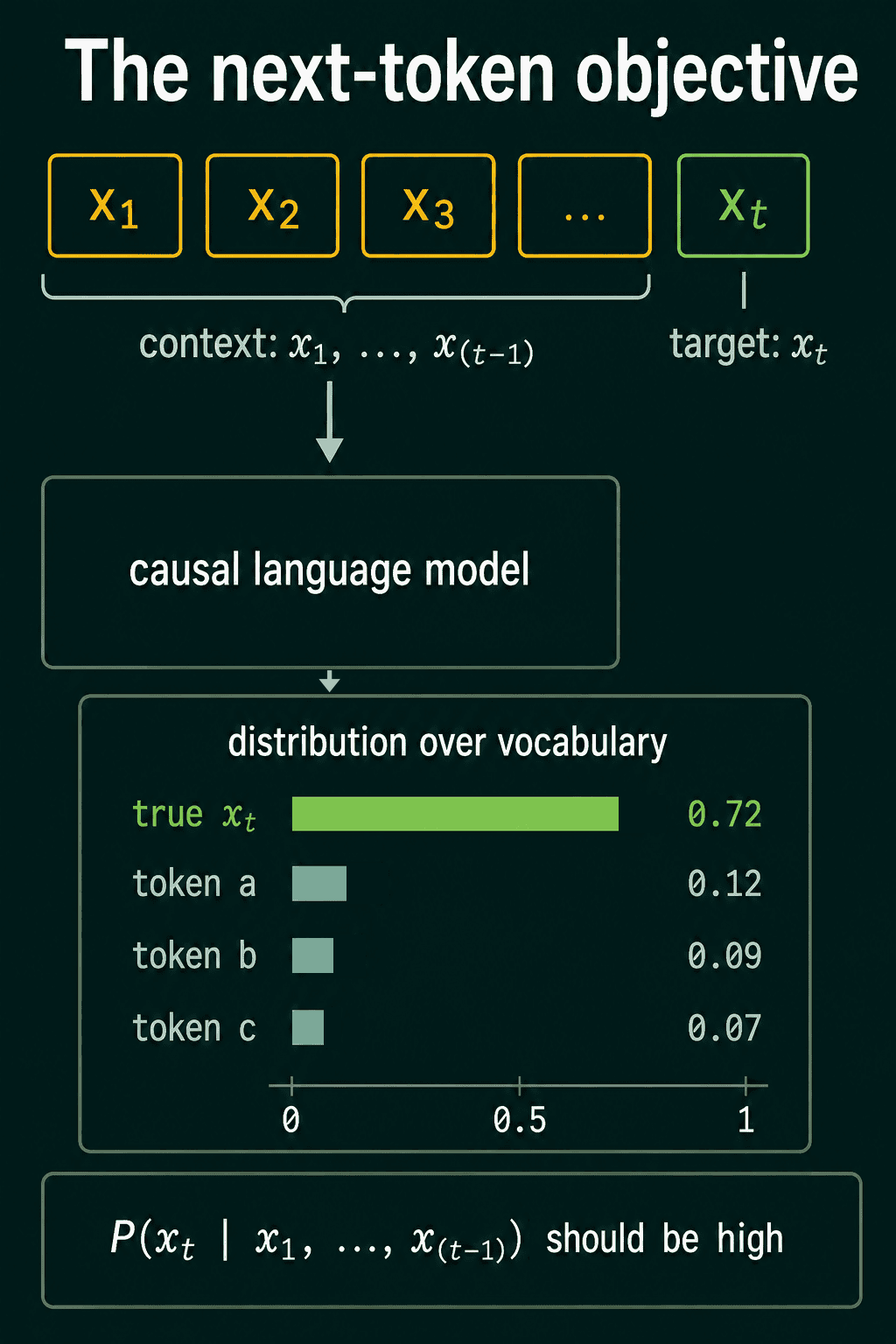
Write a piece of text as tokens $x_1, x_2, \ldots, x_t$. The tokens before position $t$ are the context, and $x_t$ is the target. A causal language model reads only the context and returns a probability for every token in its vocabulary. It is doing well at position $t$ when the probability it gives the real next token is high:

$$P(x_t \mid x_1, \ldots, x_{t-1})$$

The vertical bar reads "given", so this is the probability of $x_t$ given every token before it. That sentence is the objective. A loss function later turns it into one number that the optimizer can push down.

Context tokens x1 to x(t-1) going into a causal language model, which returns a distribution over the vocabulary with the true next token at 0.72, and the line P of x_t given the context should be high.

Where do the labels come from?

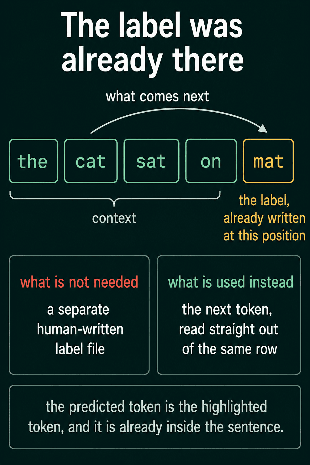
Most supervised learning needs labels written by people: this email is spam, this photo is a cat. Next-token prediction would need a label at every single position of the training text, and a training corpus can hold billions of tokens. Nobody could label that by hand.

The labels are already in the text. In the cat sat on mat, the right answer after the cat sat on is mat, and it is written right there at the next position. Training on labels read straight out of the data, with no person writing them, is called self-supervised learning. Any page of text becomes training data this way, so the amount of training signal grows with the amount of text available.

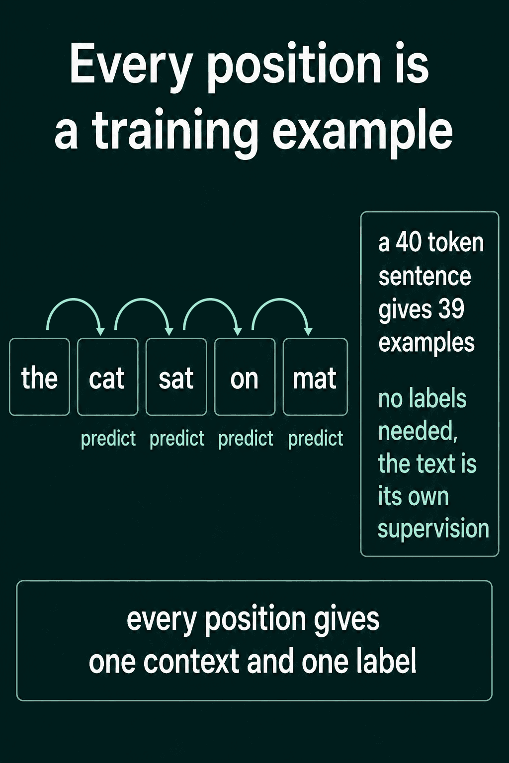
The tokens the cat sat on as context and mat highlighted as the label, already written at that position, with no separate human-written label file needed.

One sentence gives many examples, not one. The context the has the label cat, the context the cat has the label sat, and so on down the sentence. A sentence of 40 tokens gives 39 context and label pairs, one for every position after the first.

The sentence the cat sat on mat with an arrow from each token to the next, and a note that a 40-token sentence gives 39 examples.

The one-position shift

Models read token ids, not words. A tokenizer looks up each token in the vocabulary and swaps it for its number, so the cat sat on mat might become [5, 12, 47, 8, 91]. A batch of several sequences is stacked into one tensor of shape (batch, seq_len).

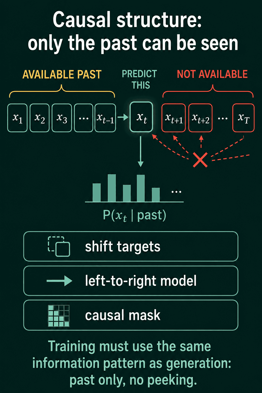
To get all the pairs at once, the input and the target are the same sequence shifted by one position. The input drops the last token, because nothing inside the sentence comes after it. The target drops the first token, because nothing predicts it:

1sentence: the cat sat on mat
2input:    the cat sat on
3target:       cat sat on mat

In PyTorch, with tokens of shape (batch, seq_len), the shift is two slices:

1input_tokens = tokens[:, :-1]   # every position except the last
2target_tokens = tokens[:, 1:]   # every position except the first

Each input position now has its label sitting at the same index in target_tokens.

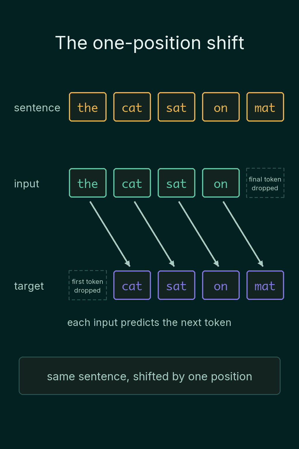
The sentence the cat sat on mat, the input row without the final token, and the target row without the first token, with each input arrow pointing to the next token.

The shift exists because of a strict rule. When a causal model predicts $x_t$, it may use only the tokens before it, never $x_t$ itself or anything after it. During generation this is automatic, since later tokens have not been written yet. During training the whole sentence sits in memory, and a model that could see the token it is supposed to predict would copy it and learn nothing. The shifted targets enforce the rule in the data, and larger models also use a causal mask, which blocks each position from attending to later ones.

Past tokens available, x_t to predict, and later tokens marked not available, with three ways to enforce it: shifted targets, a left-to-right model and a causal mask.

What is a logit?

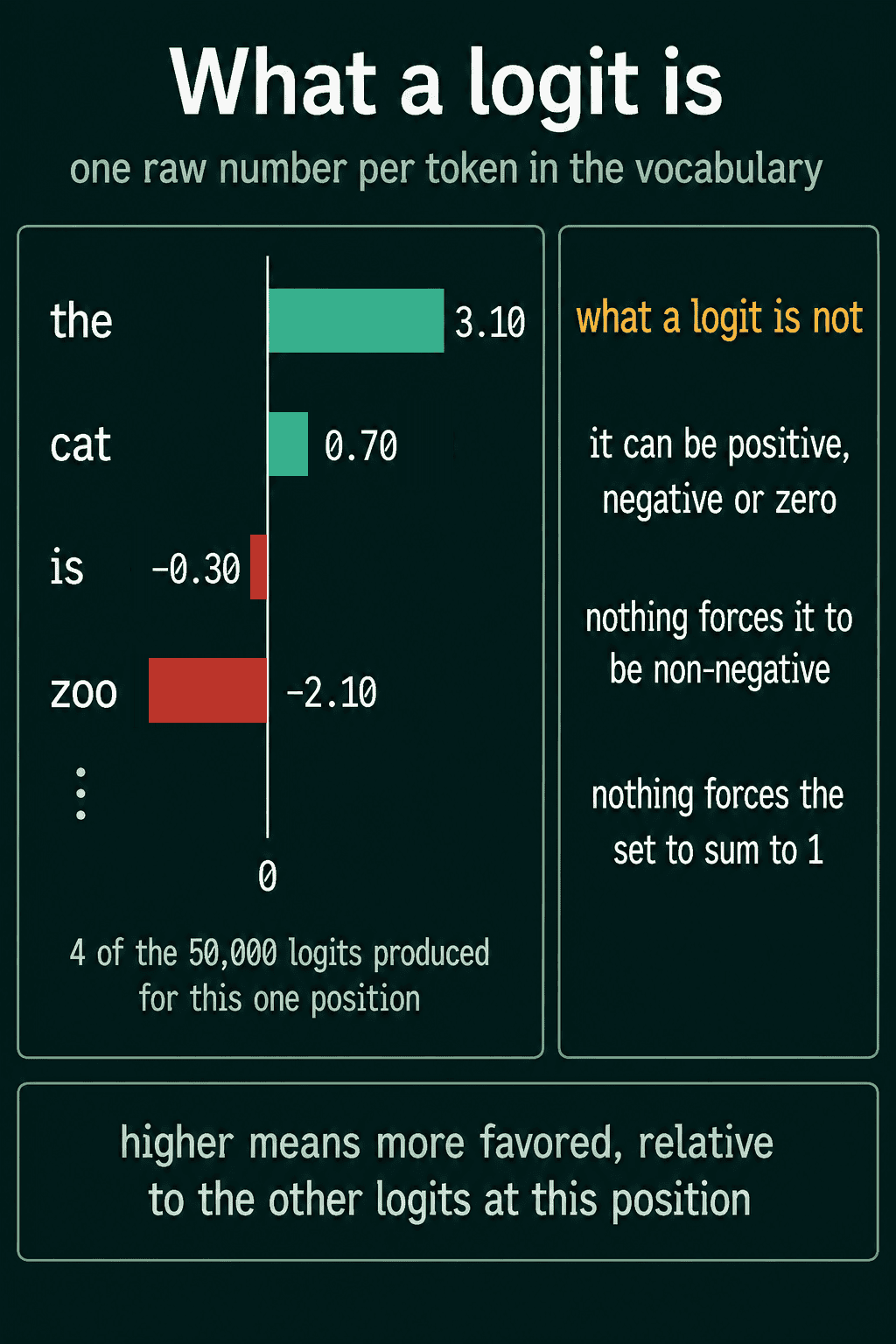
At each input position the model produces one raw score for every token in the vocabulary. If the vocabulary has 50,000 tokens, one position gets 50,000 scores, so the output tensor has shape (batch, seq_len, vocab_size).

Each raw score is called a logit. A logit can be any real number, positive, negative or zero. Nothing makes the logits add up to 1, and nothing keeps them above 0, so they are not probabilities yet. A higher logit only means the model favors that token more than the others at the same position.

Four of the 50,000 logits at one position: the at 3.10, cat at 0.70, is at -0.30 and zoo at -2.10, with notes that a logit can be negative and that the set does not sum to 1.

Softmax turns logits into probabilities

The softmax function turns the logits at one position into a probability distribution. Call $z_v$ the logit for token $v$ and $V$ the vocabulary:

$$P(x_t = v \mid x_1, \ldots, x_{t-1}) = \frac{e^{z_v}}{\sum_{v' \in V} e^{z_{v'}}}$$

The top raises $e$ to the logit of one token. The bottom does the same for every token in the vocabulary and adds the results. Raising $e$ to any number gives a positive result, so a negative logit still gets a positive probability. Dividing by the total makes the probabilities add up to exactly 1, and the token with the largest logit keeps the largest share.

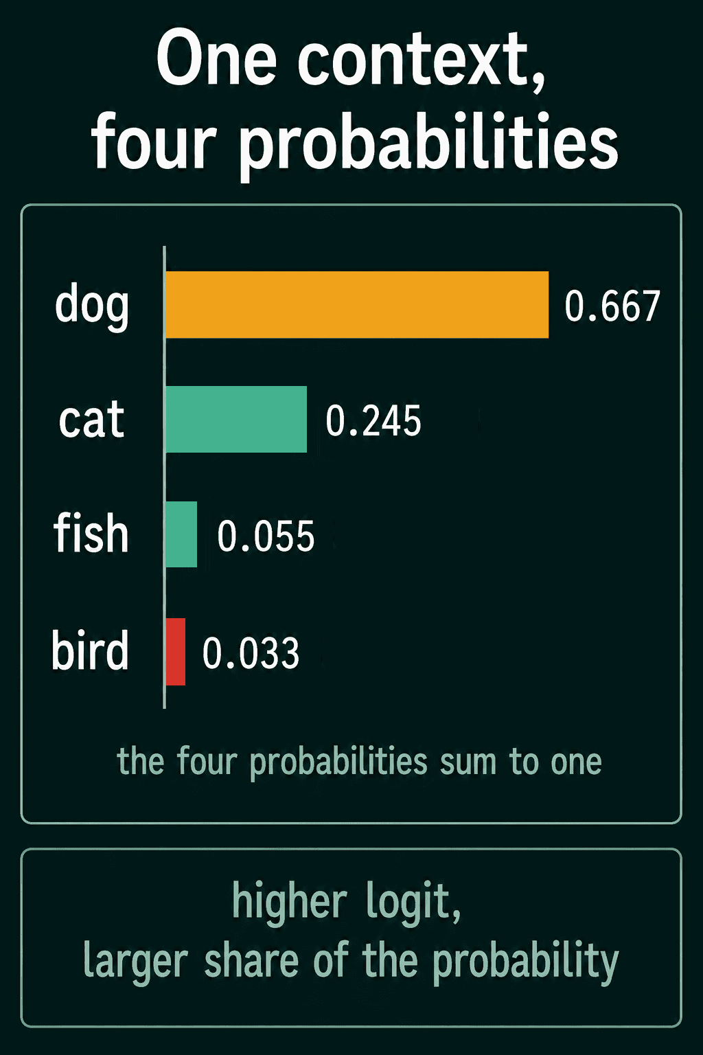
For example, take the context the child pet the and a vocabulary of only four tokens. The model returns these logits:

1dog: 2.0   cat: 1.0   fish: -0.5   bird: -1.0

Raising $e$ to each one gives $e^{2.0} \approx 7.39$, $e^{1.0} \approx 2.72$, $e^{-0.5} \approx 0.61$ and $e^{-1.0} \approx 0.37$. These add up to about 11.08. Dividing each one by 11.08 gives the probabilities. PyTorch does the same in one call:

1import torch
2import torch.nn.functional as F
3 
4logits = torch.tensor([2.0, 1.0, -0.5, -1.0])   # dog, cat, fish, bird
5probs = F.softmax(logits, dim=-1)
6print(probs.round(decimals=3))
7print(probs.sum())

1tensor([0.6670, 0.2450, 0.0550, 0.0330])
2tensor(1.)

dim=-1 applies softmax along the last axis, which is the vocabulary axis. On a real (batch, seq_len, vocab_size) tensor that gives a separate distribution at every position without changing the shape.

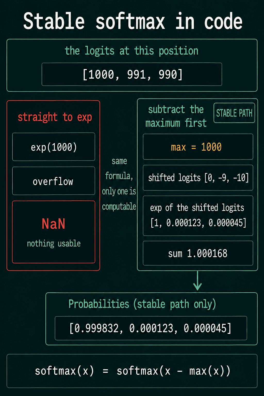
Bars for dog at 0.667, cat at 0.245, fish at 0.055 and bird at 0.033, which sum to one.

Code that computes softmax by hand usually subtracts the largest logit first. In float32, $e^{1000}$ is too large to store and becomes infinity, which turns the result into nan. Subtracting the same number from every logit cancels between the top and the bottom of the fraction, so the probabilities do not change and the largest exponent becomes $e^0 = 1$. F.softmax already does this internally.

Logits 1000, 991 and 990 overflowing when exponentiated directly, and the stable path that subtracts the maximum first and gives 0.999832, 0.000123 and 0.000045.

The loss: cross-entropy

To score a prediction, the true label is written in the same shape as the prediction: a one-hot vector $y$ with a 1 at the true token and 0 everywhere else. Call the model's probability vector $\hat p$. The standard loss for this kind of prediction is cross-entropy:

$$-\sum_{v \in V} y_v \log \hat p_v$$

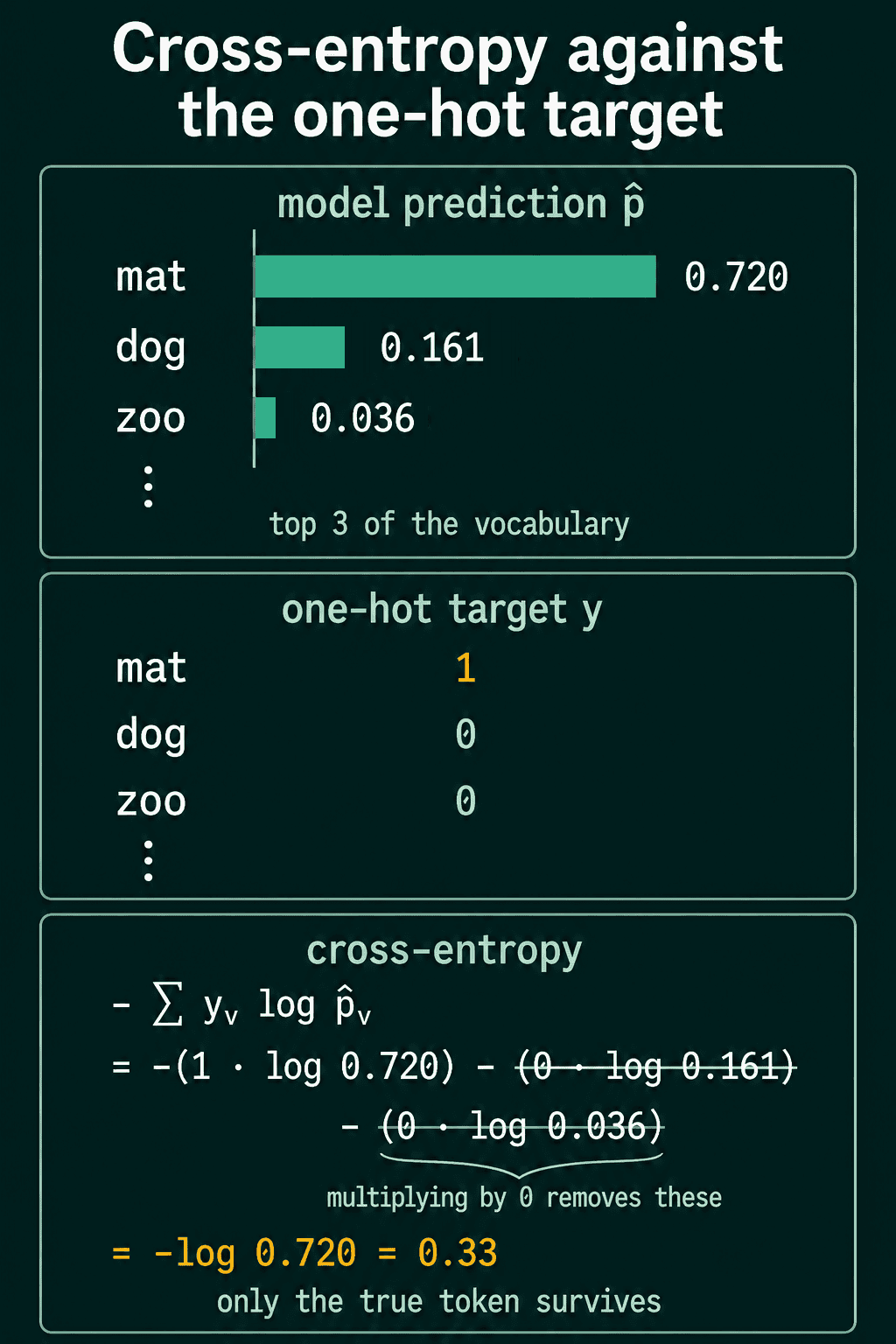
Every $y_v$ is 0 except at the true token, so every other term in the sum is multiplied by 0 and drops out. What is left is the negative log of one number:

$$-\log \hat p_{\text{true token}}$$

For example, if the true next token is mat and the model gave it probability 0.720, the loss at that position is $-\log 0.720 \approx 0.33$. A probability near 1 gives a loss near 0, and a probability near 0 gives a large loss.

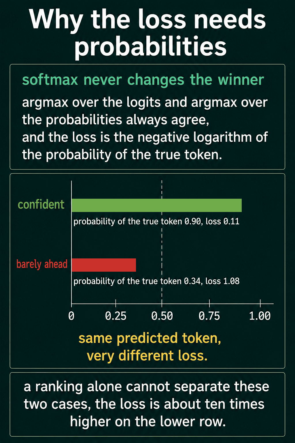
The model's probabilities mat 0.720, dog 0.161 and zoo 0.036, the one-hot target with 1 at mat, and the cross-entropy sum where the zero terms drop out, leaving -log 0.720 = 0.33.

Softmax keeps the order of the logits, so the token with the largest logit is also the most probable one. That makes it fair to ask why training does not use the logits directly. The answer is that the loss scores the probability of the true token, not its rank. A true token ranked first with probability 0.90 gets a loss of $-\log 0.90 \approx 0.11$. With probability 0.34 and two other tokens close behind, it gets $-\log 0.34 \approx 1.08$, about ten times higher. A rank cannot tell those two cases apart, and the log in the formula is undefined for the negative numbers a logit can be.

Two cases where the true token wins: probability 0.90 with loss 0.11 and probability 0.34 with loss 1.08, the same predicted token with very different loss.

Generating text by always picking the top token is called greedy decoding. For that the logits are enough, since the largest logit is also the largest probability. Methods that sample tokens at random according to their probabilities need softmax.

Cross-entropy in PyTorch takes logits

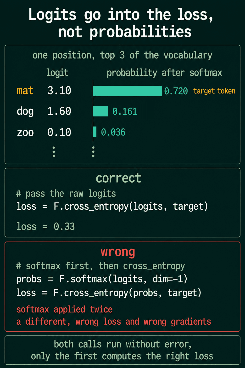
F.cross_entropy expects the raw logits, not probabilities. It applies log-softmax itself, in one numerically stable step, and then takes the negative log of the true token's probability. Passing probabilities runs softmax twice and gives a wrong loss without any error.

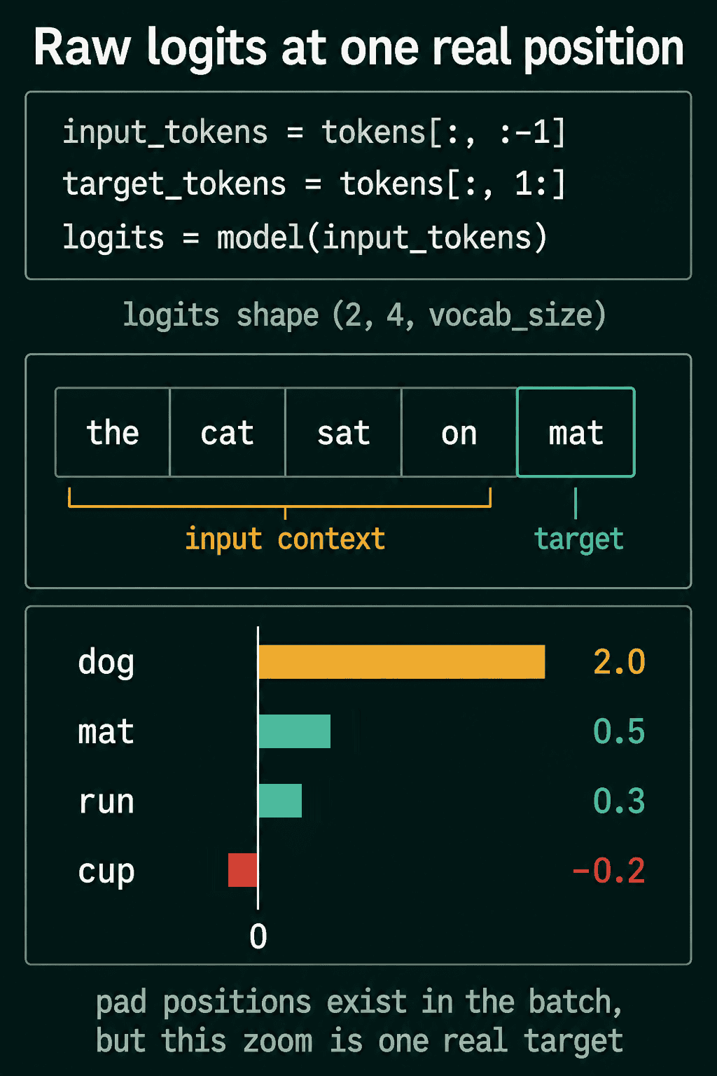
For example, take the position after the cat sat on with a four-token vocabulary of mat, dog, run and cup. The model's logits for them are 0.5, 2.0, 0.3 and -0.2. The true next token is mat:

1import torch
2import torch.nn.functional as F
3 
4logits = torch.tensor([[0.5, 2.0, 0.3, -0.2]])  # mat, dog, run, cup
5target = torch.tensor([0])                      # the true next token is mat
6 
7p_mat = F.softmax(logits, dim=-1)[0, 0]
8print(round(p_mat.item(), 3))
9print(round(-torch.log(p_mat).item(), 2))
10print(round(F.cross_entropy(logits, target).item(), 2))
11 
12probs = F.softmax(logits, dim=-1)
13print(round(F.cross_entropy(probs, target).item(), 2))   # softmax applied twice

The model gave mat probability 0.147, so the loss is $-\log 0.147 \approx 1.92$. F.cross_entropy on the logits returns the same 1.92. The last line passes probabilities instead and gets 1.52, a different number with no warning. The model is wrong here, since dog has the largest logit, and that is the kind of position where the loss is large.

The raw logits at the position after the cat sat on: dog 2.0, mat 0.5, run 0.3 and cup -0.2, with mat as the target.

The correct call passing raw logits to F.cross_entropy, and the wrong call passing softmax probabilities, which applies softmax twice and gives a wrong loss and wrong gradients.

Averaging the loss over a sequence

A training batch has many prediction positions, and F.cross_entropy scores them all in one call. It returns the average loss over the positions, which is written

$$\mathcal{L} = -\frac{1}{T}\sum_{t=1}^{T} \log P(x_t \mid x_1, \ldots, x_{t-1})$$

where $T$ is the number of scored positions. Each term is the loss at one position, and the average is the single number that training lowers.

Real sentences have different lengths, but a batch has to be a rectangular tensor. Shorter sequences get a special pad token added at the end until every row is as long as the longest one. A pad token is not real text, so the model should not be rewarded or punished for predicting it. Passing ignore_index with the pad id leaves those positions out of the average.

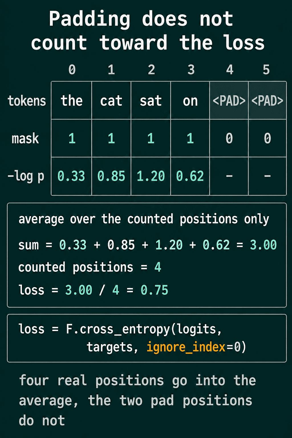
Tokens the cat sat on followed by two pad tokens, a mask of four 1s and two 0s, per-position losses 0.33, 0.85, 1.20 and 0.62, and the loss averaged over the four real positions only: 3.00 / 4 = 0.75.

A full training step in PyTorch

The code below puts every piece together on two sentences, the cat sat on mat and the shorter she runs fast, padded with id 0. The model is the smallest neural language model there is: an embedding table that turns each token id into 32 learned numbers, and a linear layer that turns those numbers into one logit per vocabulary token. It sees only the current token, so it can learn which token tends to follow which, and nothing longer.

1import torch
2import torch.nn as nn
3import torch.nn.functional as F
4 
5torch.manual_seed(0)
6vocab_size, pad_id = 100, 0
7 
8# two sentences as token ids, the second padded with 0
9tokens = torch.tensor([
10    [5, 12, 47, 8, 91],   # the cat sat on mat
11    [33, 61, 27, 0, 0],   # she runs fast <pad> <pad>
12])
13 
14input_tokens = tokens[:, :-1]    # (2, 4)
15target_tokens = tokens[:, 1:]    # (2, 4)
16 
17model = nn.Sequential(
18    nn.Embedding(vocab_size, 32),
19    nn.Linear(32, vocab_size),
20)
21optimizer = torch.optim.Adam(model.parameters(), lr=0.01)
22 
23for step in range(201):
24    logits = model(input_tokens)                  # (2, 4, vocab_size)
25    loss = F.cross_entropy(
26        logits.reshape(-1, vocab_size),
27        target_tokens.reshape(-1),
28        ignore_index=pad_id,
29    )
30    optimizer.zero_grad()
31    loss.backward()
32    optimizer.step()
33    if step % 50 == 0:
34        print(step, round(loss.item(), 3))
35 
36probs = F.softmax(model(input_tokens), dim=-1)
37print(round(probs[0, 3, 91].item(), 3))   # P(mat | ... on)

The reshape calls flatten the batch and position axes, so every position becomes one row of 100 logits with one target id. Before any training the loss is 4.51, close to $\ln 100 \approx 4.6$, which is the loss of a model that spreads its probability evenly over 100 tokens. The three lines inside the loop are one training step: zero_grad() clears the gradients left from the last step, backward() computes how each weight should move to lower the loss, and step() moves every weight a small amount in that direction. After 200 steps the model gives mat probability 0.998 after on. The loss falls almost to 0 because the model memorized two sentences, which says nothing about how it would handle new text.

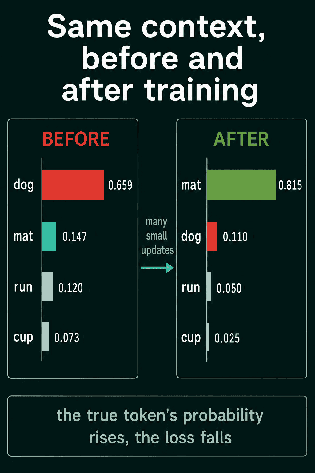
Each step moves the weights only a little. On the earlier example, many small updates move the logits at the position after the cat sat on until mat is the most probable token instead of dog. The loss at that position drops from 1.92 to $-\log 0.815 \approx 0.20$.

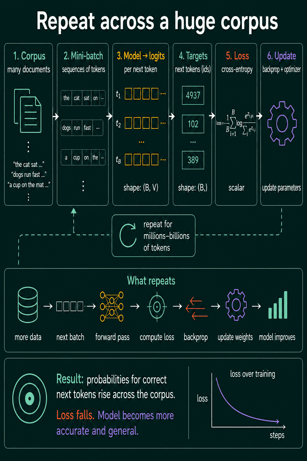
Before training, dog at 0.659 and mat at 0.147, and after many small updates, mat at 0.815 and dog at 0.110: the true token's probability rises and the loss falls.

A real model repeats this over billions of tokens of text. Patterns that show up across many different texts, such as which words follow which or how verbs agree with their subjects, push the weights in the same direction again and again. A phrase that appears once has much less effect. That is why a trained model can give sensible next-token probabilities for a sentence it never saw: it learned patterns that many sentences share, not one particular sentence.

The training loop over a large corpus: mini-batches, model to logits, next-token targets, cross-entropy loss and a weight update, repeated over millions to billions of tokens while the loss falls.

From next-token predictions to a sentence's probability

Training scores one position at a time, but evaluation often asks a different question: how likely is a whole sentence? Counting whole sentences in a corpus does not work, because almost any sentence longer than a few tokens appears zero times.

The chain rule of probability builds the whole-sequence probability out of next-token pieces. For two tokens, $P(a, b) = P(a)\, P(b \mid a)$: the chance of the first token times the chance of the second one given the first. For a longer sequence the same step repeats, with each token conditioned on everything before it:

$$P(x_1, x_2, \ldots, x_T) = \prod_{t=1}^{T} P(x_t \mid x_1, \ldots, x_{t-1})$$

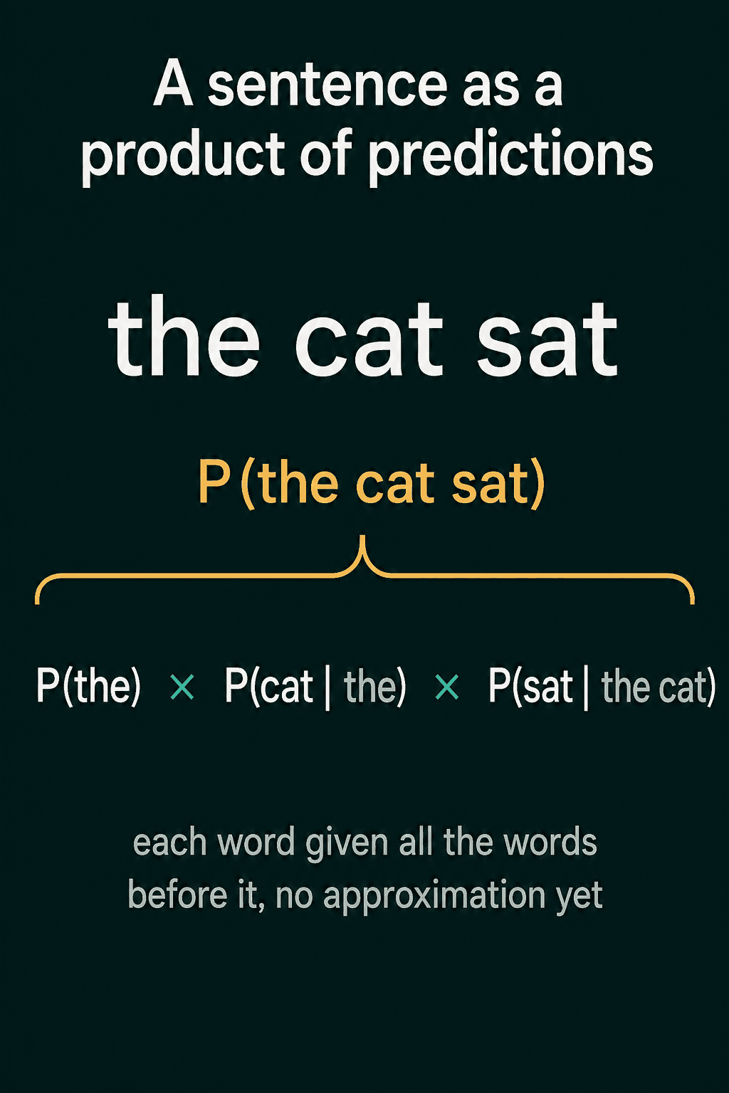
The $\prod$ symbol means multiply all the terms together. For example, $P(\text{the cat sat}) = P(\text{the}) \cdot P(\text{cat} \mid \text{the}) \cdot P(\text{sat} \mid \text{the cat})$. This is exact, with no approximation, and every factor is the quantity a causal language model predicts. So a model that predicts next tokens can also score any sequence.

The sentence the cat sat, with P(the cat sat) split into P(the) times P(cat given the) times P(sat given the cat).

In code the product is computed as a sum of log probabilities, because multiplying many numbers below 1 quickly gets too small for a float to hold. The model scores each token given the ones before it, and the function adds up the log probability of each true next token:

1import torch
2import torch.nn as nn
3import torch.nn.functional as F
4 
5def sequence_logprob(model, tokens):
6    logits = model(tokens[:, :-1])
7    targets = tokens[:, 1:]
8    log_probs = F.log_softmax(logits, dim=-1)
9    picked = log_probs.gather(-1, targets.unsqueeze(-1)).squeeze(-1)
10    return picked.sum(dim=-1)
11 
12torch.manual_seed(0)
13model = nn.Sequential(nn.Embedding(100, 32), nn.Linear(32, 100))
14tokens = torch.tensor([[5, 12, 47, 8, 91]])
15score = sequence_logprob(model, tokens)
16print(score.shape, round(score.item(), 2), torch.exp(score).item())

1torch.Size([1]) -18.22 1.2270517935064618e-08

At every position gather picks the log probability stored at the true next token's id. unsqueeze(-1) adds the extra axis that gather expects and squeeze(-1) removes it again. The untrained model gives this sentence a log probability of -18.22, which is a probability of about 0.00000001. Like the training code, it scores the four tokens after the first one.

Common mistakes

Passing probabilities to F.cross_entropy. It applies its own log-softmax, so softmaxing first gives a wrong loss and wrong gradients with no error.
Forgetting the shift. Comparing logits with tokens instead of tokens[:, 1:] trains the model to predict the token it was just given.
Counting padding in the loss. Without ignore_index, the model is trained to predict pad tokens and the average loss mixes in positions that are not text.
Writing softmax by hand without subtracting the maximum. Large logits overflow to infinity and the result becomes nan.
Multiplying many probabilities to score a long sequence. The product falls below what a float can hold, so add log probabilities instead.

The language model post covers what a language model outputs and how a bigram model gets its probabilities by counting instead of training. Averaging the per-token loss and raising $e$ to it gives perplexity, the usual way to compare language models on a test set. The model in the training code above sees one token at a time, and a recurrent neural network is the simplest model that carries information from earlier tokens forward.

QuiddityML teaches next-token training as four concepts in the language models unit of its NLP track. Its exercises include filling in the one-position shift, saying what goes wrong when probabilities are passed to F.cross_entropy and writing the language modeling loss from scratch (QuiddityML).