By Sagi Shaier · 2 November 2026 · 12 min read

What is a language model? From bigrams to neural next-token prediction

What a language model outputs and what it is used for, how a bigram model builds its probabilities by counting in Python, and why neural models replaced the counting.

A language model assigns probabilities to the next token, the unit of text a model reads and predicts, which can be a whole word or a piece of one. Given the tokens so far, it returns a probability for every token it knows, saying how likely each one is to come next. Chat assistants, autocomplete, translation and summarization all rely on models trained on this task or a close relative of it.

A different job for token vectors

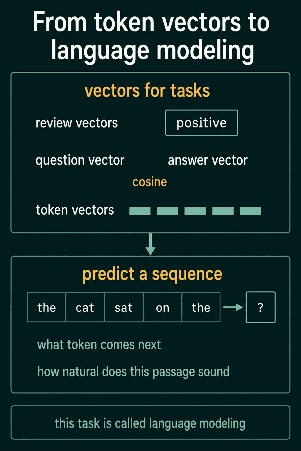
Once tokens are turned into vectors of numbers, those vectors support many tasks. A review can be classified as positive or negative, and a question vector can be compared with an answer vector to find the best match. Language modeling uses them for something else: following a sequence as it unfolds. Given the cat sat on the, which token should come next? And how natural does a whole passage sound?

What does a language model output?

Most modern models split text into tokens that are subword pieces rather than whole words, so unbelievable might become un, believ and able. That keeps the list of tokens a manageable size and still covers words the model never saw whole.

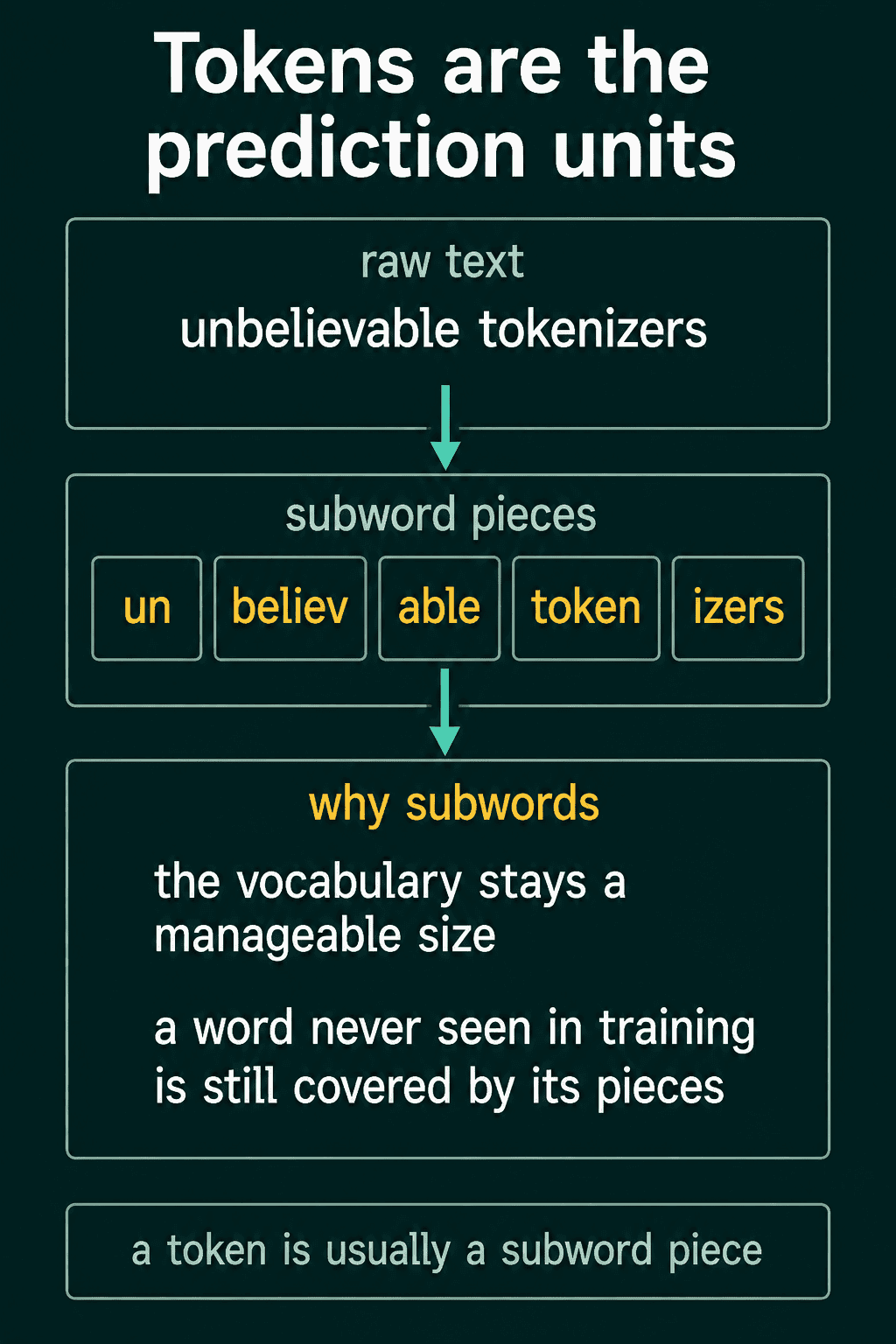
The full list of tokens a model knows is its vocabulary, written $V$. For one position in the text, a language model returns a probability for every token in $V$. If the vocabulary has 50,000 tokens, the output is 50,000 numbers that are all at least 0 and add up to 1.

A causal language model, also called autoregressive, predicts from left to right. Call the tokens seen so far $x_1, \ldots, x_{t-1}$ and the next token $x_t$. For every token $v$ in the vocabulary, the model returns the probability that the next token is $v$, given everything before it:

$$P(x_t = v \mid x_1, \ldots, x_{t-1})$$

For example, if the text so far is the cute, a model might return:

1P(axolotl | the cute) = 0.42
2P(cat      | the cute) = 0.18
3P(puppy    | the cute) = 0.11
4... many other vocabulary tokens

Many chat models are causal language models.

A masked language model predicts a hidden token inside the sentence instead of the next one. Given the [MASK] axolotl, it sees words on both sides of the gap and returns a probability for each token that could fill it, such as cute at 0.37 and tiny at 0.21. BERT is the classic example. A masked model is usually not used to write text one token at a time.

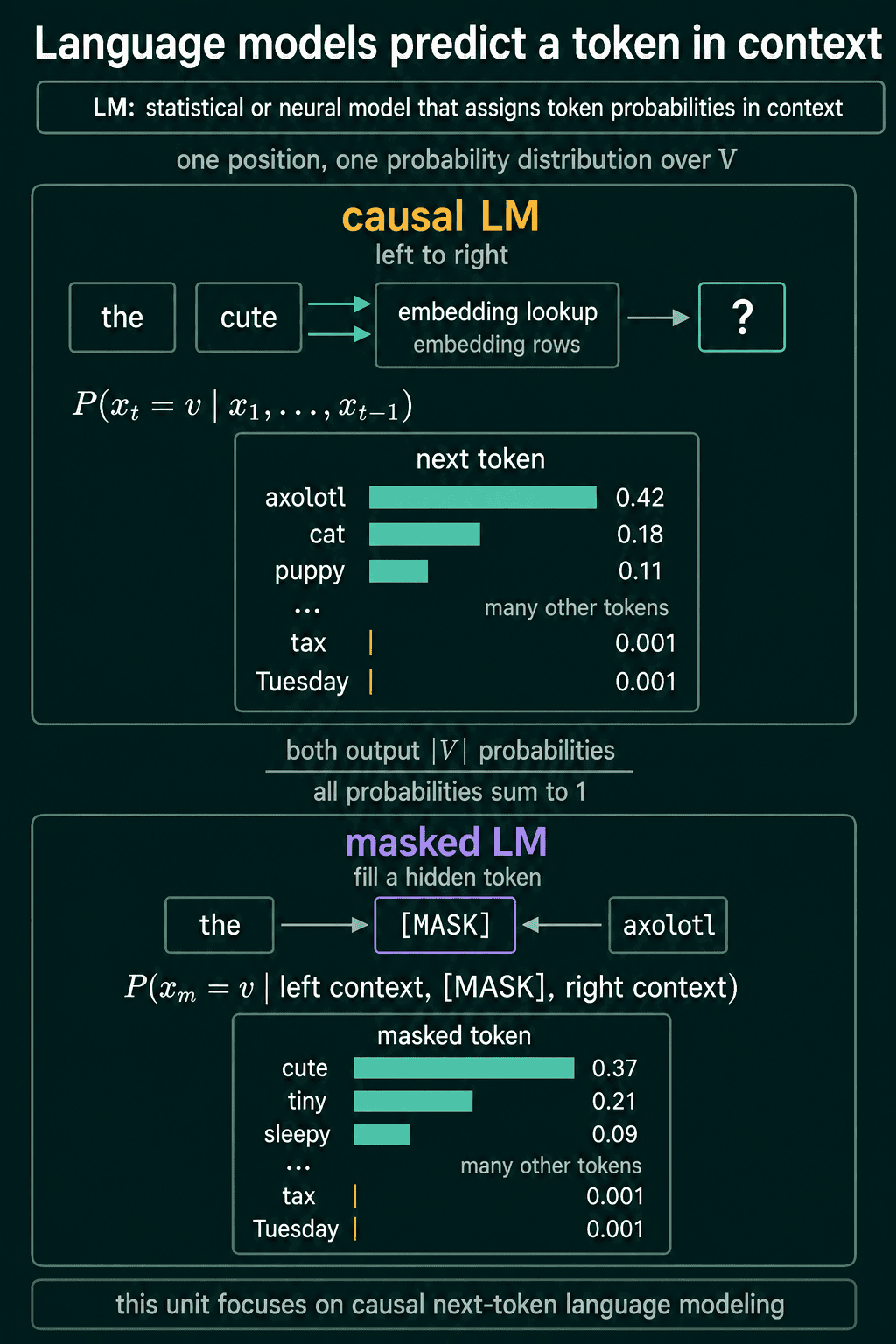
The rest of this post is about causal language models.

What are language models used for?

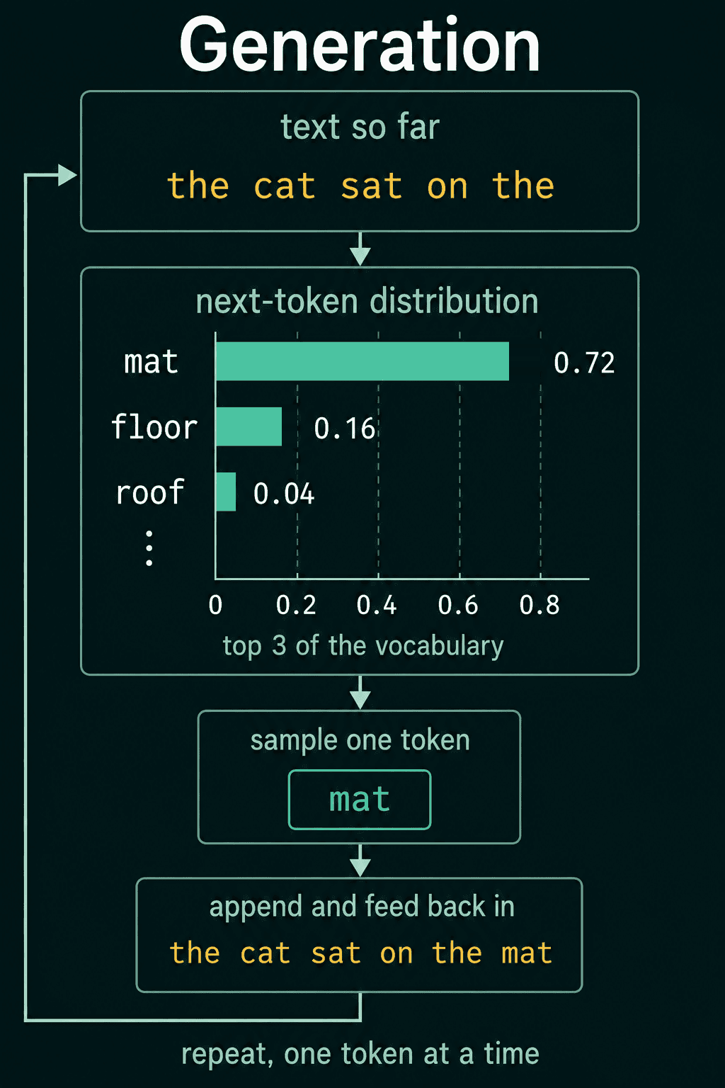
Writing text. If a model can predict the next token, it can write. Pick a token from the next-token probabilities, add it to the text, then feed the longer text back in and pick again. Repeating this produces new text one token at a time, which is what a chatbot reply or an autocomplete suggestion is doing. How the token gets picked from the probabilities is a separate choice, called decoding.

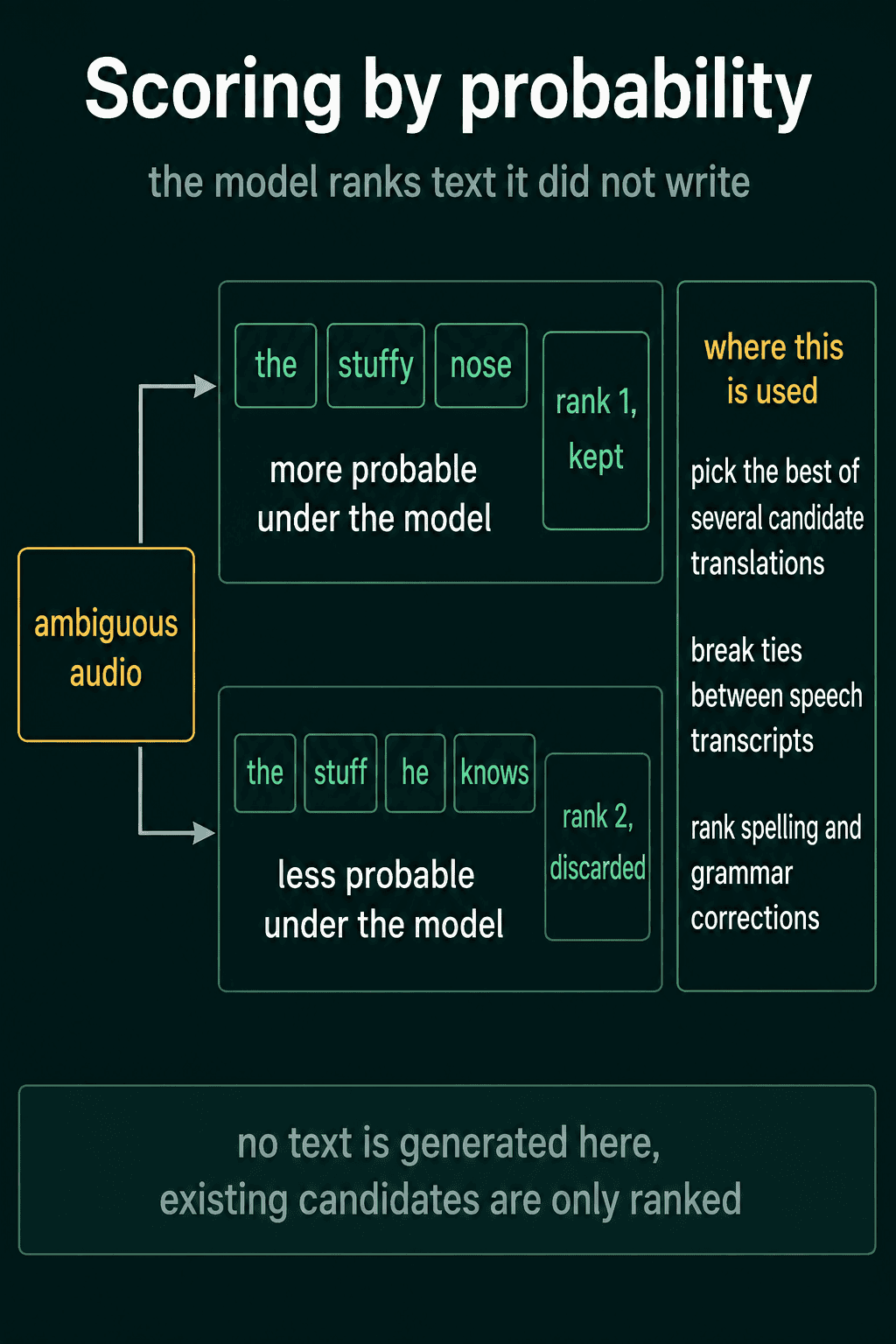
Scoring text. A causal language model can also score text without writing any. Combining the next-token probabilities across a sequence gives one probability for the whole sequence, so several candidates can be ranked against each other. A speech recognizer that hears an unclear stretch of audio might produce both the stuffy nose and the stuff he knows. The language model breaks the tie by giving a higher probability to the one that better matches the text it was trained on. Translation systems pick between candidate translations the same way, and spelling and grammar checkers rank their corrections with it.

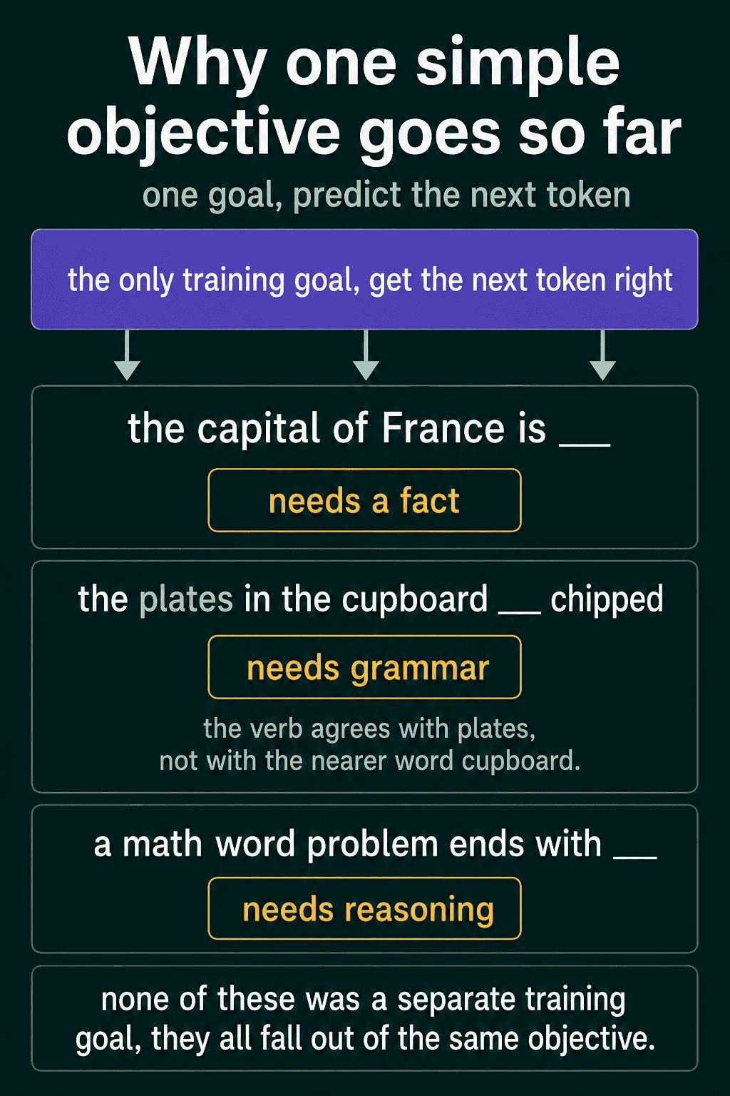
Predicting the next token sounds too simple to support all of this. It works because predicting well forces a model to pick up many kinds of structure. To finish the capital of France is ___ it needs a fact. To choose the verb in the plates in the cupboard ___ chipped it needs grammar, because the verb has to agree with plates and not with the nearer word cupboard. To finish a math word problem it needs some reasoning. None of these was a separate training goal.

Why can't a model count the whole history?

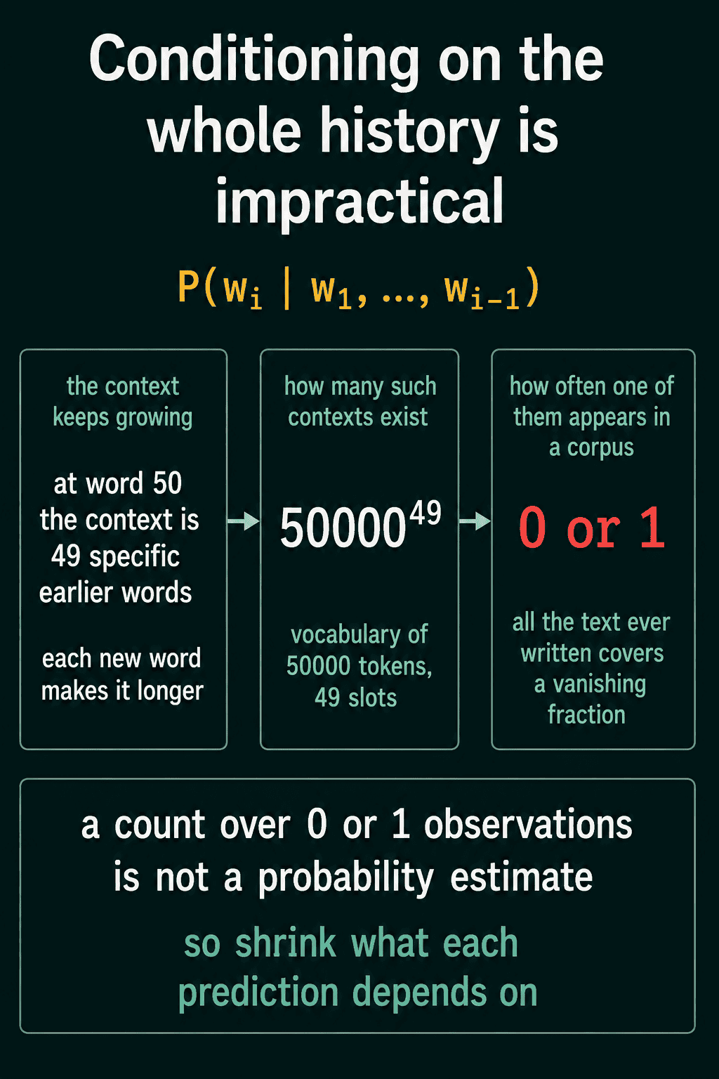
The most direct way to get next-token probabilities is to count: look up every time the same context appeared in a large amount of text, and count what came next. The problem is that the context keeps growing. By word 50 the context is 49 specific earlier words. With a vocabulary of 50,000 tokens there are $50000^{49}$ possible 49-word contexts, far more than all the text ever written could cover. Any particular 49-word context will show up zero times or once, and a count of zero or one is not a probability you can use.

The Markov assumption: keep only the recent past

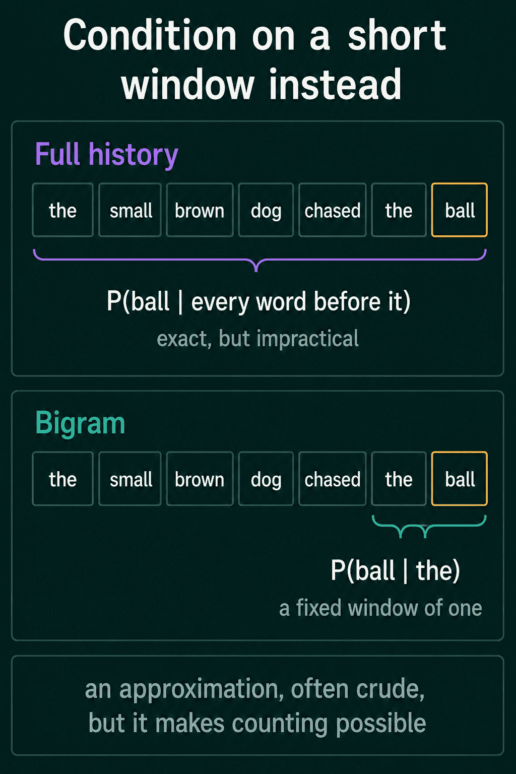
The Markov assumption fixes this by keeping only the last few tokens of the context. The examples from here on use whole words as tokens to keep them simple. The simplest useful version is the bigram assumption: the next word depends only on the one word right before it.

$$P(w_i \mid w_1, \ldots, w_{i-1}) \approx P(w_i \mid w_{i-1})$$

Here $w_i$ is the word at position $i$. The left side conditions on every earlier word, and the right side keeps only the previous one. In the small brown dog chased the ball, the full history for ball is six words, and the bigram keeps only the. It throws away most of the context, and in exchange the probability becomes something you can count.

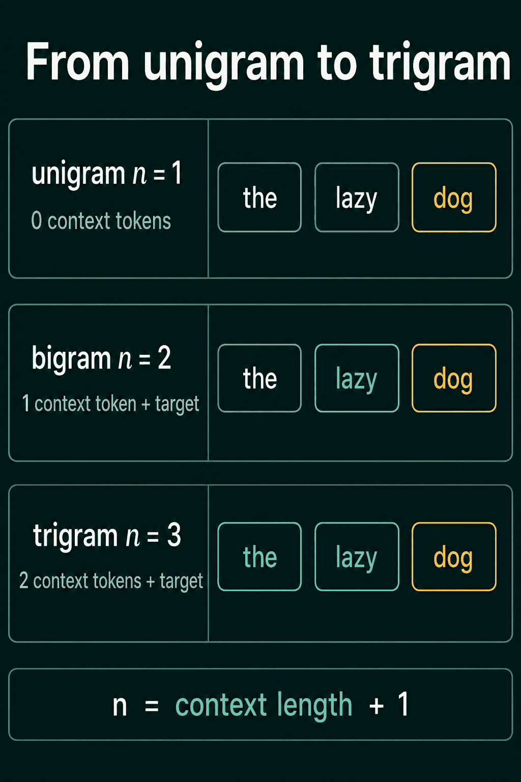
Keeping the previous $n - 1$ tokens is called an n-gram assumption, where $n$ counts the predicted token plus its context:

• unigram ($n = 1$): no context, only how common each token is
• bigram ($n = 2$): the previous 1 token
• trigram ($n = 3$): the previous 2 tokens

So a trigram estimate of $P(\text{barks} \mid \text{the dog})$ uses the two-word context the dog and ignores everything before it.

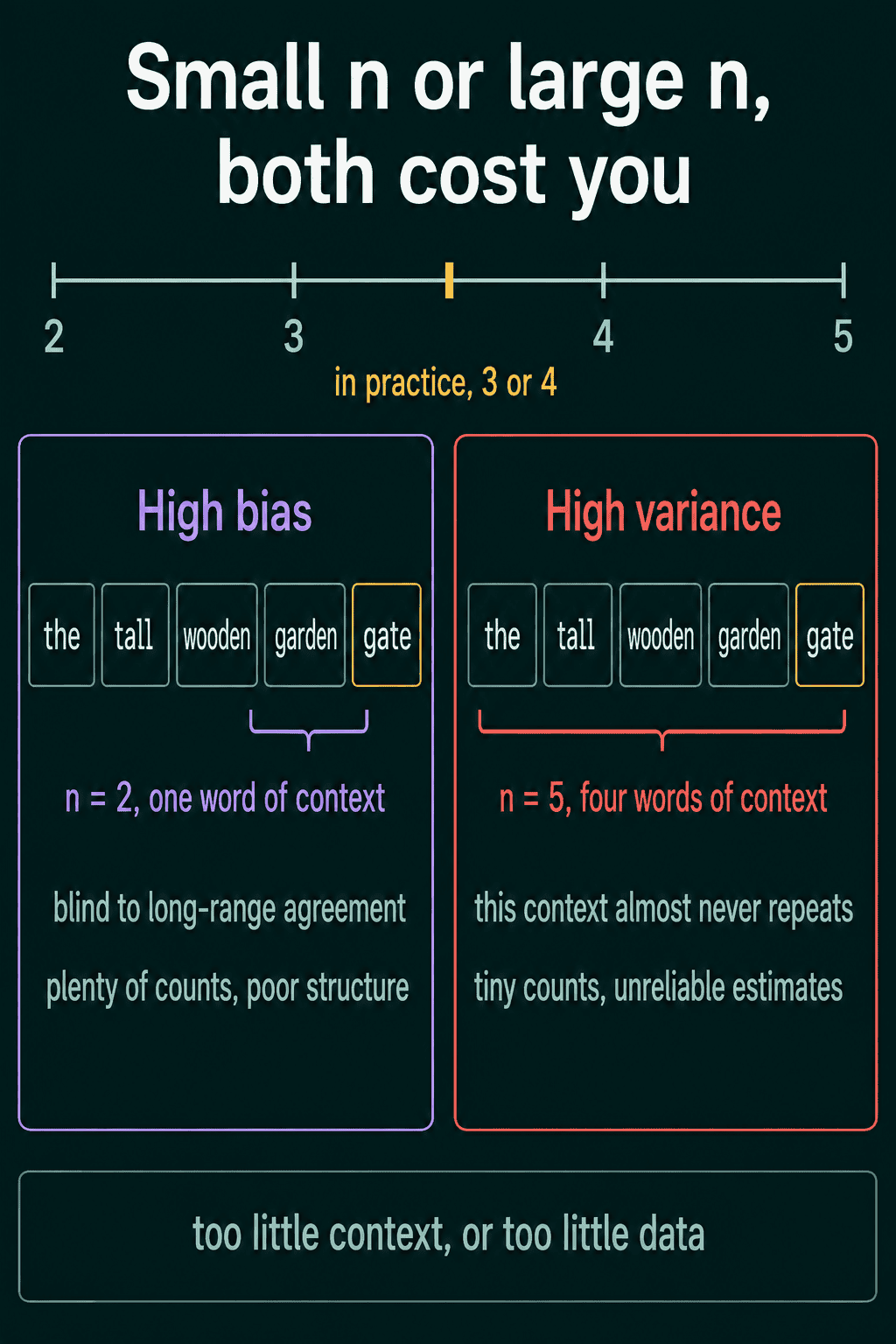
Picking $n$ trades two problems against each other. A small $n$ sees too little: a bigram cannot make a verb agree with a subject several words back, because that subject is outside its one-word window. This kind of error, built into the model's limited view, is called high bias. A large $n$ sees enough but has too little data: a 5-gram context like the small brown spotted almost never repeats in training text, so its counts are tiny and its estimates jump around. That is high variance. In practice trigrams and 4-grams were common.

How does a bigram model work?

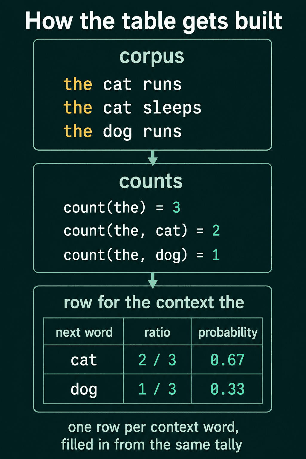
A bigram model gets its probabilities by counting word pairs in a collection of text, called a corpus. No weights are trained. The finished model is a table: one row per context word, and in each row the probability of every word that can follow it.

Take a tiny corpus of three sentences:

1the cat runs
2the cat sleeps
3the dog runs

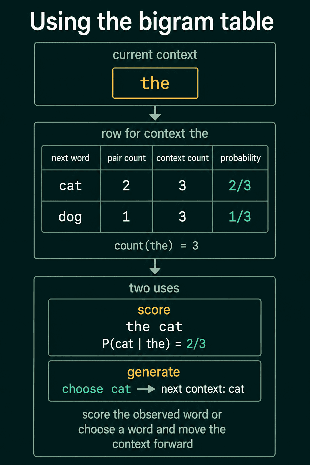
The word the appears 3 times. It is followed by cat twice and by dog once. So the probability that cat follows the is 2 out of 3, and the probability of dog is 1 out of 3:

$$P(\text{cat} \mid \text{the}) = \frac{2}{3}, \qquad P(\text{dog} \mid \text{the}) = \frac{1}{3}$$

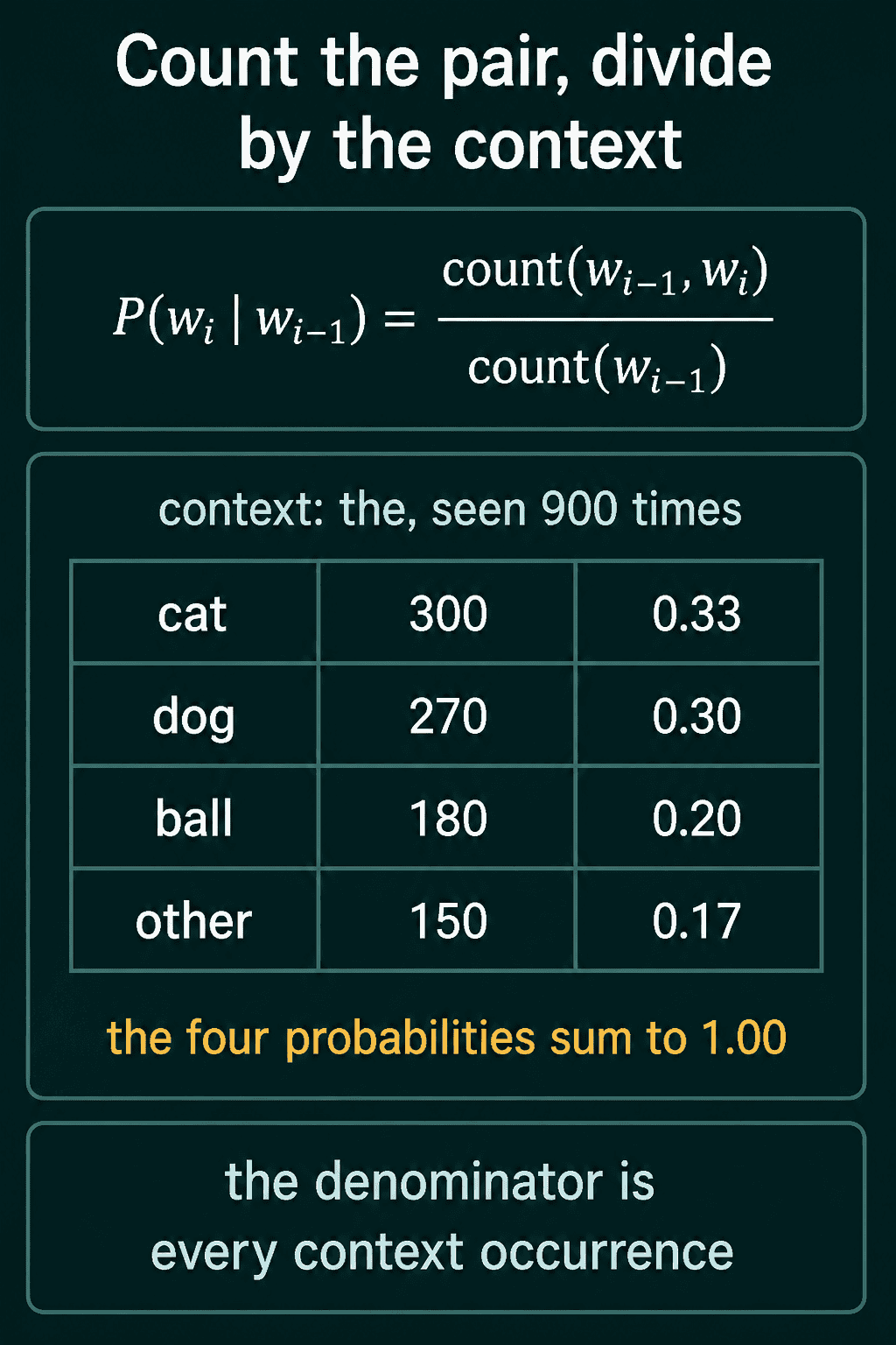
The general rule counts how often the pair appeared and divides by how often the context word appeared:

$$P(w_i \mid w_{i-1}) = \frac{\text{count}(w_{i-1}, w_i)}{\text{count}(w_{i-1})}$$

Because the bottom of the fraction is every appearance of the context word, the probabilities in one row add up to 1. In a larger corpus where the appears 900 times and is followed by cat 300 times, $P(\text{cat} \mid \text{the}) = 300 / 900 = 0.33$.

Estimating a probability as how often something happened in the data has a name: maximum likelihood estimation, or MLE. These count ratios are the probabilities that make the training corpus as likely as possible.

Marking where sentences start and end

The first word of a sentence has no word before it, and nothing in the table says when a sentence is over. Counting toolkits fix both by adding two extra tokens to every sentence, one at the start and one at the end. With the markers added, the start marker is followed by the 3 times out of 3, so $P(\text{the} \mid \text{START}) = 1$. The word runs is followed by the end marker both times it appears. The counts inside each sentence stay the same, so $P(\text{cat} \mid \text{the})$ is still $2/3$.

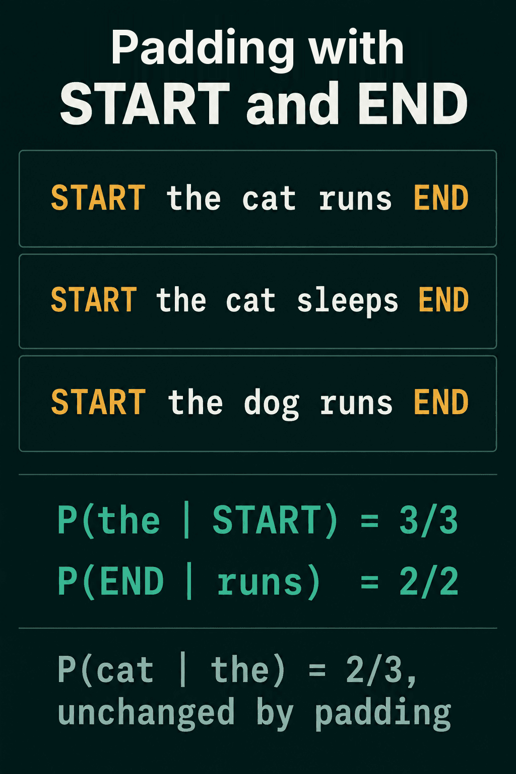
In code the markers are usually written <s> and </s>. Python's Counter does the tallying, since it starts every missing key at 0. The second function scores a sentence by multiplying its bigram probabilities:

1from collections import Counter
2 
3def bigram_probs(corpus):
4    bigram_counts = Counter()
5    context_counts = Counter()
6    for sentence in corpus:
7        toks = ['<s>'] + sentence.split() + ['</s>']
8        for i in range(1, len(toks)):
9            bigram_counts[(toks[i - 1], toks[i])] += 1
10            context_counts[toks[i - 1]] += 1
11    return {(prev, w): c / context_counts[prev] for (prev, w), c in bigram_counts.items()}
12 
13corpus = ["the cat runs", "the cat sleeps", "the dog runs"]
14probs = bigram_probs(corpus)
15print(round(probs[('the', 'cat')], 2), round(probs[('the', 'dog')], 2))
16print(probs[('<s>', 'the')], probs[('runs', '</s>')])
17 
18def sentence_prob(sentence, probs):
19    toks = ['<s>'] + sentence.split() + ['</s>']
20    p = 1.0
21    for prev, w in zip(toks, toks[1:]):
22        p *= probs.get((prev, w), 0.0)   # an unseen pair gets probability 0
23    return p
24 
25print(round(sentence_prob("the dog runs", probs), 3))
26print(round(sentence_prob("the cat runs", probs), 3))
27print(sentence_prob("the dog sleeps", probs))

10.67 0.33
21.0 1.0
30.333
40.333
50.0

the dog runs gets $1 \times 1/3 \times 1 \times 1 = 0.333$. the cat runs gets $1 \times 2/3 \times 1/2 \times 1$, which is also 0.333. The last line comes out as exactly 0, because the pair dog sleeps never appeared in the corpus.

Using the table to write text

Writing text is a walk through the table. Start at <s> and pick the next word from that row using its probabilities. Then move to the row for the word you picked, and stop when you reach </s>:

1import random
2from collections import Counter
3 
4def bigram_probs(corpus):
5    bigram_counts = Counter()
6    context_counts = Counter()
7    for sentence in corpus:
8        toks = ['<s>'] + sentence.split() + ['</s>']
9        for i in range(1, len(toks)):
10            bigram_counts[(toks[i - 1], toks[i])] += 1
11            context_counts[toks[i - 1]] += 1
12    return {(prev, w): c / context_counts[prev] for (prev, w), c in bigram_counts.items()}
13 
14probs = bigram_probs(["the cat runs", "the cat sleeps", "the dog runs"])
15 
16def generate(probs):
17    word, out = '<s>', []
18    while True:
19        row = {w: p for (prev, w), p in probs.items() if prev == word}   # the row for the current word
20        word = random.choices(list(row), weights=list(row.values()))[0]
21        if word == '</s>':
22            return ' '.join(out)
23        out.append(word)
24 
25random.seed(0)
26for _ in range(5):
27    print(generate(probs))

1the dog runs
2the cat sleeps
3the cat sleeps
4the dog runs
5the dog runs

The model can also write the cat runs, but never the dog sleeps, because every step has to follow a pair it saw.

Where counting breaks

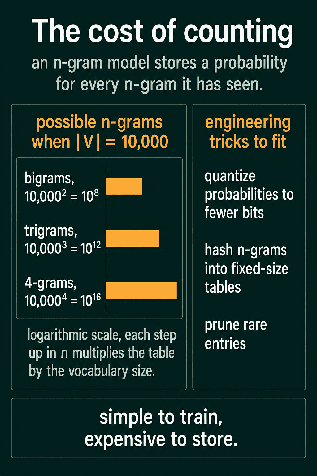
Storage. An n-gram model stores a probability for every n-gram it has seen, and the number of possible n-grams grows very fast with $n$. With a vocabulary of 10,000 words there are $10000^2 = 10^8$ possible bigrams, $10^{12}$ trigrams and $10^{16}$ 4-grams. Real n-gram systems fit in memory with tricks such as storing probabilities with fewer bits, hashing n-grams into a fixed-size table, and dropping rare entries.

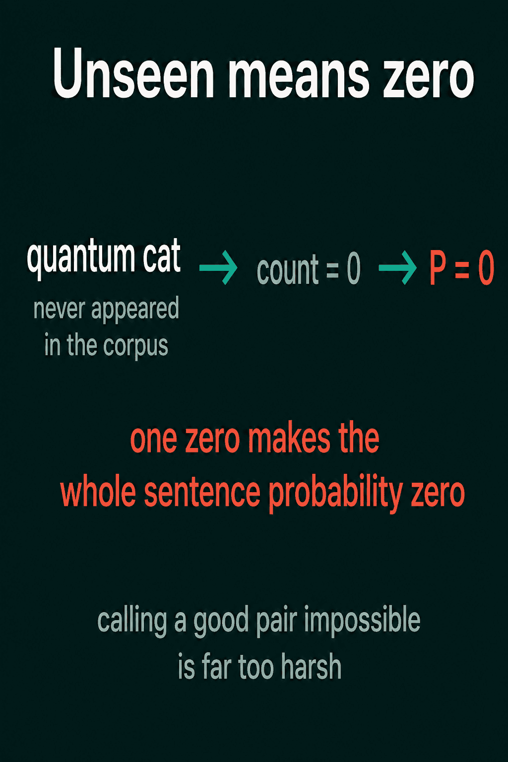
Unseen pairs get zero. Any n-gram that never appeared in training gets a count of 0, so the counting rule gives it probability 0. Plenty of normal word pairs happen to be missing from any particular corpus, and treating them as impossible is wrong. A sentence's probability is a product of its n-gram probabilities, so one zero makes the whole sentence's probability zero, as the dog sleeps showed above.

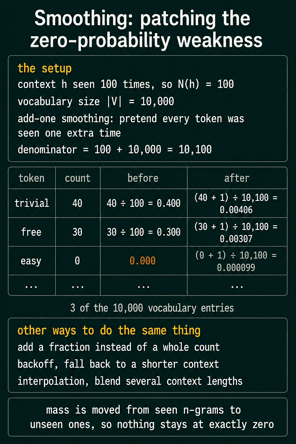
A family of fixes called smoothing moves a little probability from the n-grams that were seen to the ones that were not. Add-one smoothing pretends every possible word was seen one extra time after each context. For example, say a context appeared 100 times and the word free followed it 30 times, with a vocabulary of 10,000 words. Without smoothing $P = 30 / 100 = 0.3$. With add-one smoothing every count gets 1 added and the bottom grows by 10,000, so $P = 31 / 10100 = 0.00307$. A word that never followed the context now gets $1 / 10100 = 0.000099$ instead of 0. Other methods add a smaller amount, fall back to a shorter context when the longer one was never seen (backoff), or blend estimates from several context lengths (interpolation).

From counting to neural language models

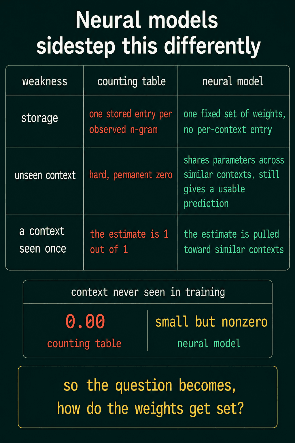
A neural language model avoids both problems differently. It has one fixed set of weights instead of a stored entry per n-gram, so the table-size problem goes away. And because it shares its weights across similar contexts, it can still give a sensible prediction for a context it never saw exactly, instead of a hard zero.

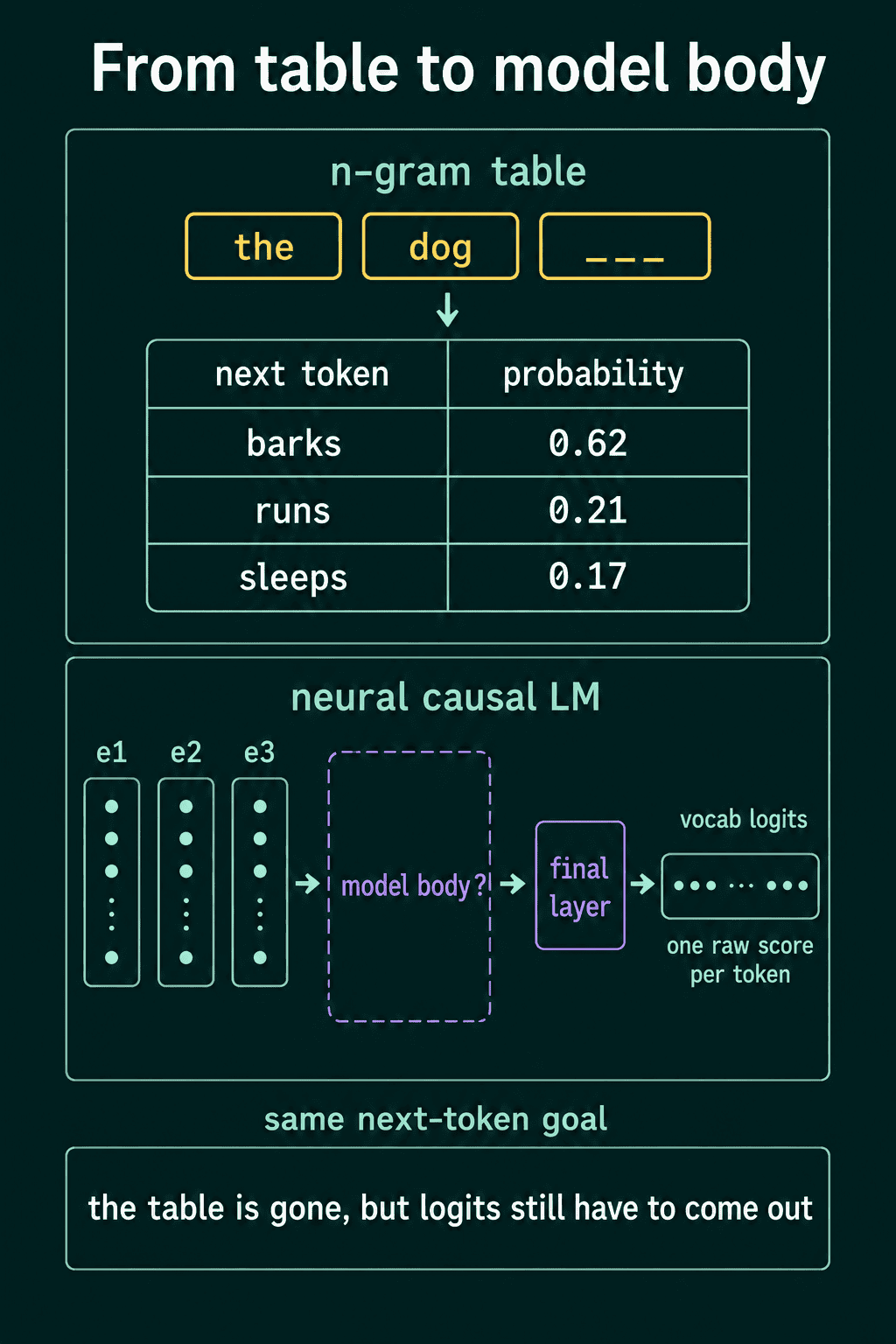
A neural causal language model keeps the same output goal as the table. At each position it produces one raw score per vocabulary token, called a logit, and a final step turns those scores into probabilities. What changes is the part in between, the model body, which reads the token vectors and has to produce something the final layer can score.

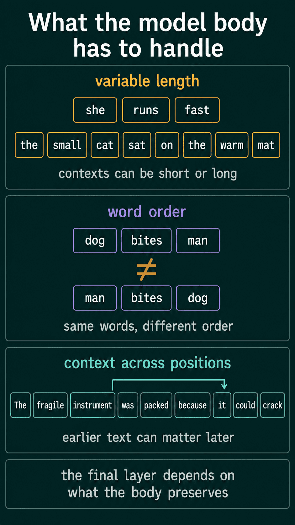
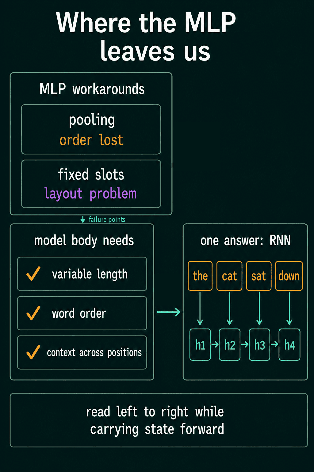
That body has to handle three things about language at once. Contexts can be short or long. Order changes meaning, since dog bites man and man bites dog use the same words. And information has to travel across positions: in The violinist wrapped the fragile instrument in extra padding because it could crack, the word it refers back to instrument, not violinist.

A basic feedforward network called an MLP is the natural first try. It expects an input of fixed size, and text arrives in any length. There are two workarounds, and each one loses something:

• Average the token vectors into one. Any length becomes one vector of the same size. But the average does not depend on order, so the cat chased the dog and the dog chased the cat look identical, even though the next word should differ.
• Give the MLP a fixed number of slots, one per position, and pad or cut every input to that length. Order survives, but the network has separate weights for each slot, so a pattern learned near the start of the text does not carry over to the same pattern later on.

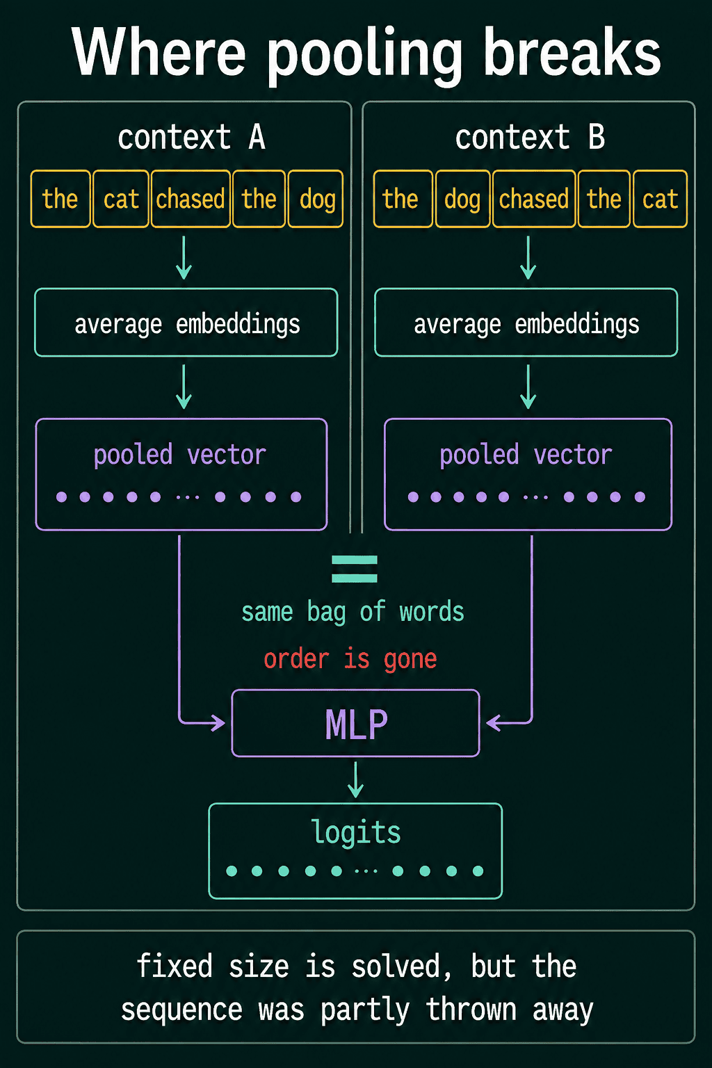
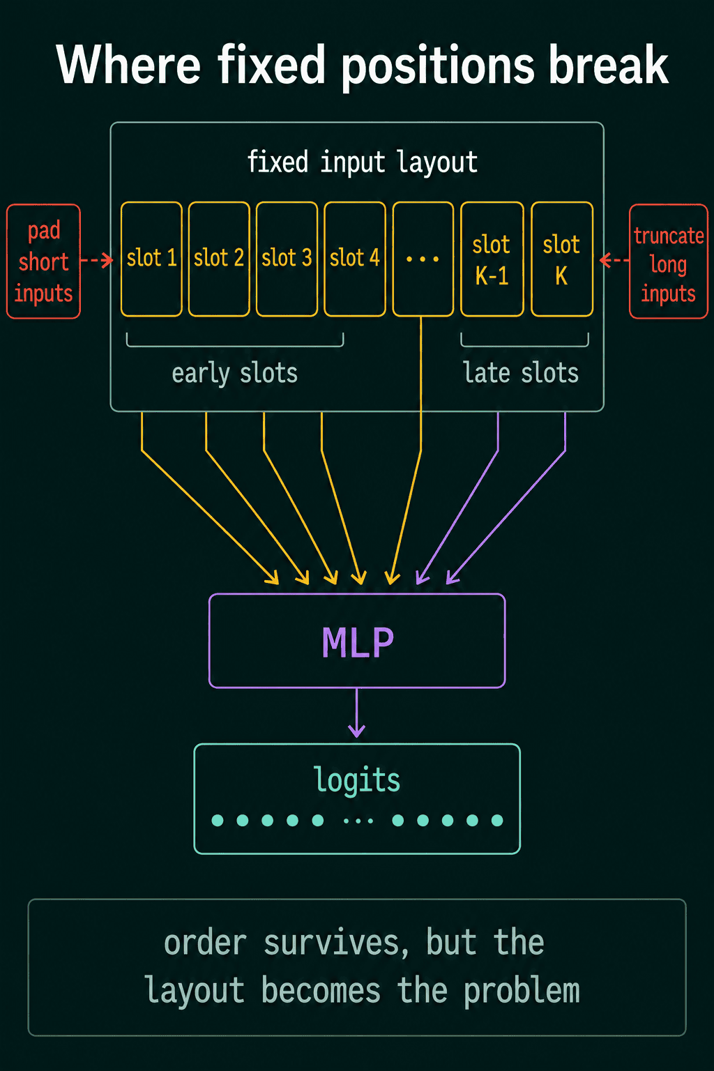
Neither workaround gives a clean way to carry information from early positions to later ones. The design that follows is to read the text left to right and carry a running summary forward, updating it at each token. A recurrent neural network, or RNN, is the simplest model built that way.

Common mistakes

• Using a masked model as a text writer. A masked model fills gaps from both sides, and it is not built to predict the next token from the left only.
• Mixing up $n$ and the context length. A trigram uses 2 context tokens, because $n$ includes the predicted token.
• Leaving out the start and end markers. Without them the first word has no context and the model has no way to learn where sentences stop.
• Scoring sentences with unsmoothed counts. One unseen pair gives the whole sentence a probability of 0, so smooth before scoring.
• Choosing a large $n$ for a small corpus. Longer contexts repeat rarely, and their estimates come from one or two examples.

Related concepts

Language models predict tokens, and the tokenization post covers how text gets split into them. Neural language models start from token vectors, which the word embeddings post explains, and the static vs contextual embeddings post covers why a word's vector should depend on its sentence.

QuiddityML teaches language models from the bigram table up in the language models unit of its NLP track, and the exercises include filling in the blanks of the bigram counting function, tracing its counts on a three-sentence corpus and writing it from scratch (QuiddityML).