By Sagi Shaier · 3 November 2026 · 14 min read

Recurrent neural networks (RNNs) explained, with backpropagation through time

The RNN update worked by hand, then coded from scratch and with nn.RNN, plus how backpropagation through time trains it, why its gradients vanish or explode, and what bidirectional and stacked RNNs change.

A recurrent neural network (RNN) reads a sequence one element at a time. It carries a vector of numbers called the hidden state from each step to the next. At every step it combines the current input with the hidden state from the step before and writes a new hidden state. RNNs were a common neural model for text and speech before transformers, and they are the simplest neural model that reads text in order while keeping track of what came earlier.

What problem does an RNN solve?

Text is a sequence of tokens, the units a model reads, which can be whole words or pieces of words. Each token is first turned into a vector of numbers, called its embedding. The examples below treat each word as one token to keep them simple.

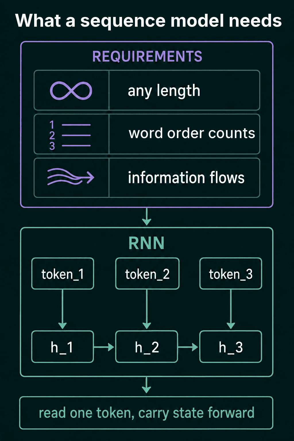
A model that reads text has to handle three things. Inputs come in any length, from 3 tokens to 3,000. Order changes meaning, since dog bites man and man bites dog contain the same words. And information has to travel from early tokens to later ones, so that a word near the end can depend on one near the start.

A plain feedforward network expects an input of fixed size, so it handles none of these directly. An RNN handles all three with one idea: read left to right, and at each position update a running summary of everything read so far.

The three needs of a sequence model, any length, word order and information flowing forward, met by an RNN that reads token 1, 2 and 3 and passes hidden states h1 to h2 to h3.

The hidden state

That running summary is the hidden state, a vector with a fixed number of entries. After reading the, the model has one hidden vector. After reading cat, it has a new one, computed from the embedding of cat and the vector it had after the. After sat, it updates again.

Every position uses the same pattern: current token in, previous hidden state in, new hidden state out. The word recurrent means this same update is reused at each position, which is why the model can keep going for 3 tokens or 300.

The RNN update rule

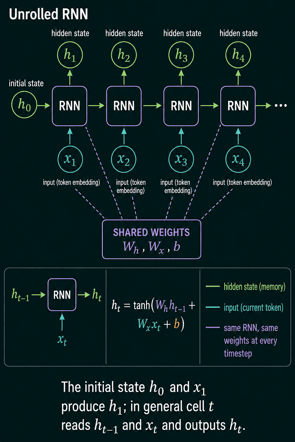
At position $t$ the update has two inputs:

$\mathbf{x}_t$, the embedding of the current token.
$\mathbf{h}_{t-1}$, the hidden state from the previous position.

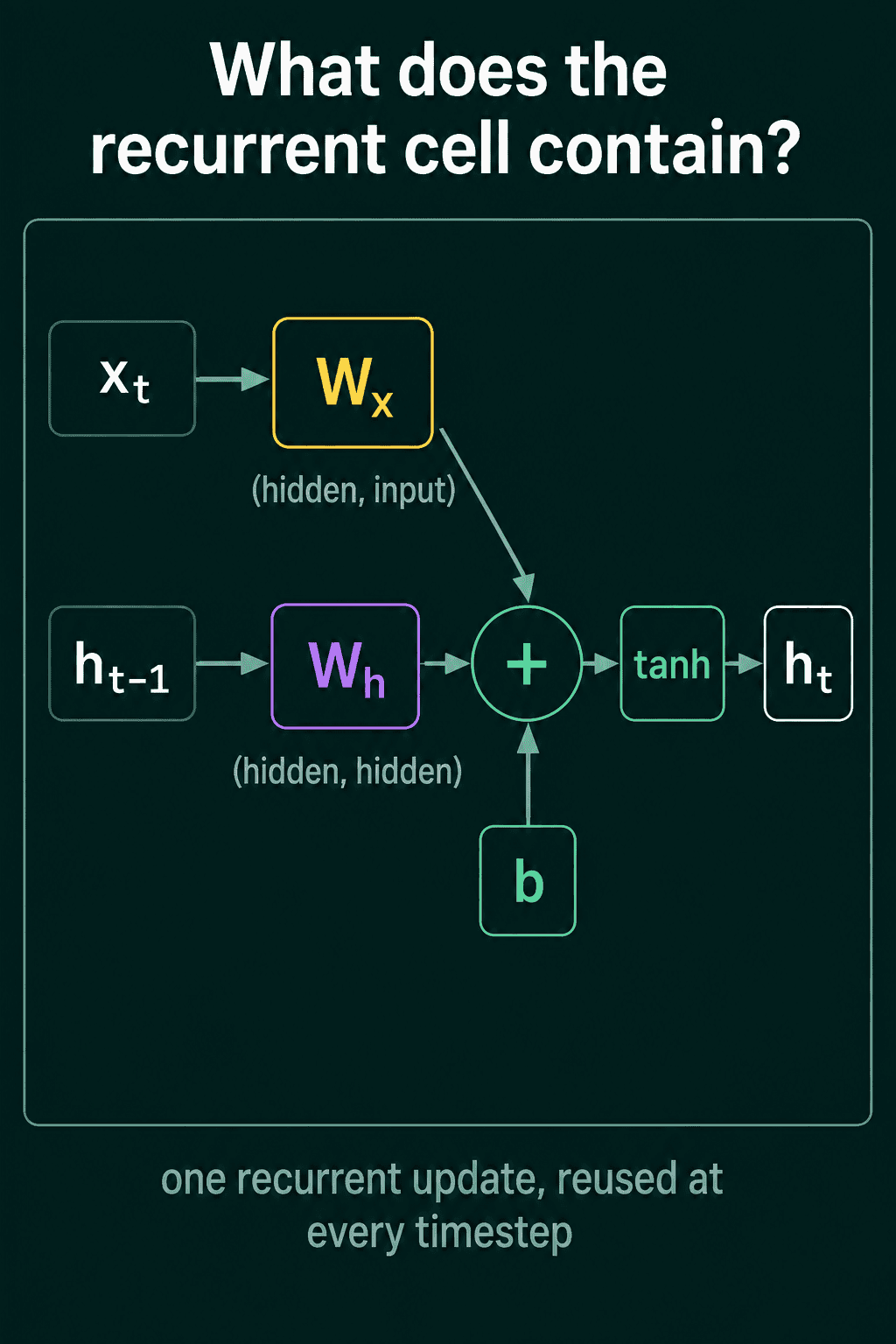
It multiplies each input by its own learned matrix and adds a learned bias vector $\mathbf{b}$. The sum goes through tanh, a function that squashes every number into the range from -1 to 1:

$$\mathbf{h}_t = \tanh(\mathbf{W}_h \mathbf{h}_{t-1} + \mathbf{W}_x \mathbf{x}_t + \mathbf{b})$$

The same $\mathbf{W}_h$, $\mathbf{W}_x$ and $\mathbf{b}$ are used at every position. Sharing them across positions is what lets one model handle sequences of any length. The first hidden state $\mathbf{h}_0$ is usually a vector of zeros.

An RNN unrolled over four tokens, starting from h0, with the same shared weights W_h, W_x and b used at every step, and the update h_t = tanh(W_h h_(t-1) + W_x x_t + b).

These are the only learned parts of the recurrent update. With embeddings of size input_size and a hidden state of size hidden_size:

$\mathbf{W}_x$ has shape (hidden_size, input_size) and is applied to the current token embedding.
$\mathbf{W}_h$ has shape (hidden_size, hidden_size) and is applied to the previous hidden state.
$\mathbf{b}$ has shape (hidden_size,) and is added before tanh.

A full language model built on an RNN also has an embedding table before it and a layer after it that turns each hidden state into one score per vocabulary token. The RNN is the middle part that carries context through the sequence.

The recurrent cell: x_t through W_x of shape (hidden, input), h_(t-1) through W_h of shape (hidden, hidden), both added with b, then tanh gives h_t.

One step by hand

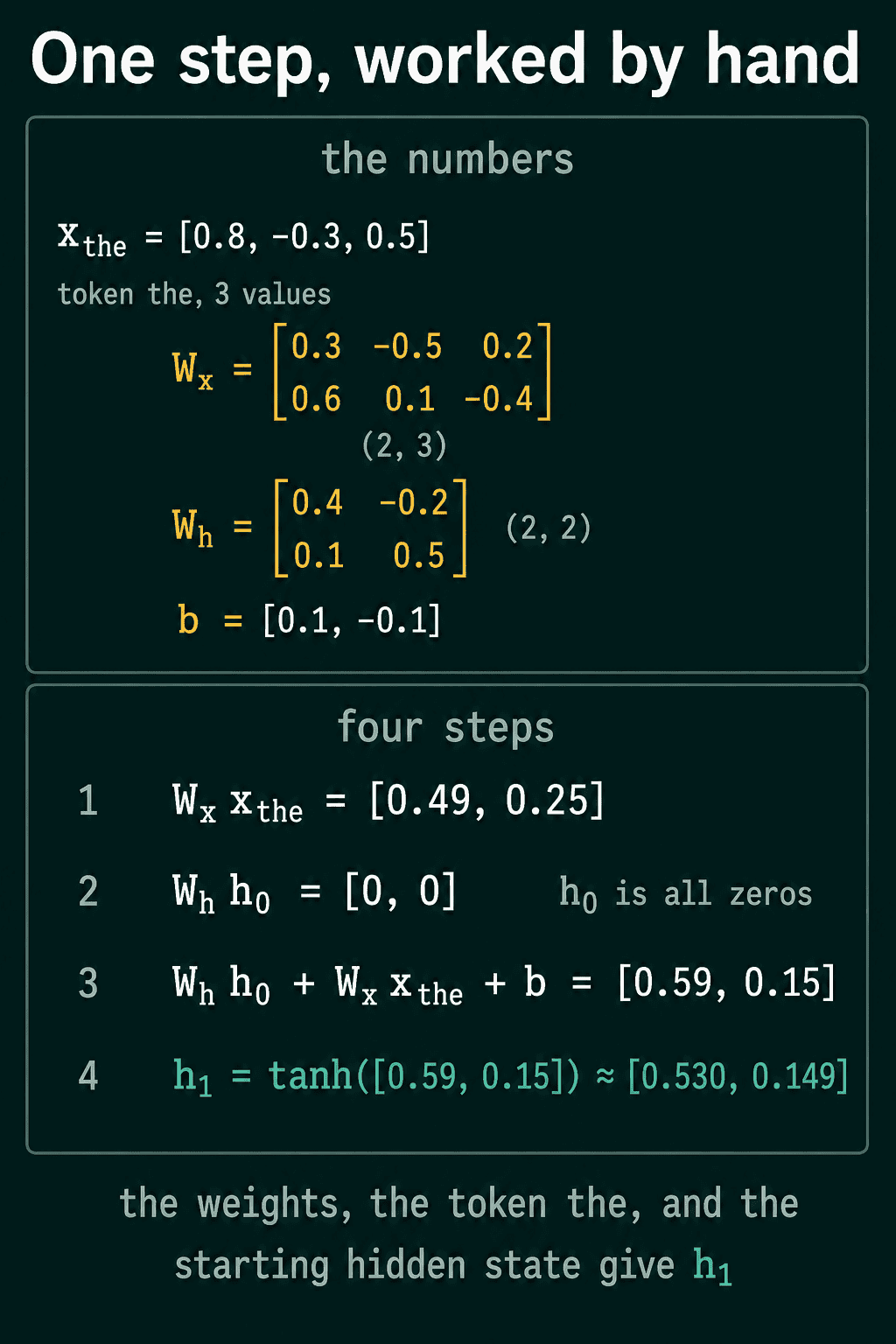
Take the sentence the cat sat with embeddings of 3 numbers and a hidden state of 2 numbers, so input_size = 3 and hidden_size = 2. That makes $\mathbf{W}_x$ shape (2, 3), $\mathbf{W}_h$ shape (2, 2) and $\mathbf{b}$ shape (2,):

$$\mathbf{W}_x = \begin{pmatrix} 0.3 & -0.5 & 0.2 \\ 0.6 & 0.1 & -0.4 \end{pmatrix}, \quad \mathbf{W}_h = \begin{pmatrix} 0.4 & -0.2 \\ 0.1 & 0.5 \end{pmatrix}$$

$$\mathbf{b} = [0.1,\ -0.1]$$

The embedding of the is $\mathbf{x}_{\text{the}} = [0.8, -0.3, 0.5]$, and the starting hidden state is $\mathbf{h}_0 = [0, 0]$. Each row of $\mathbf{W}_x$ times $\mathbf{x}_{\text{the}}$ gives one entry: $0.3 \cdot 0.8 - 0.5 \cdot (-0.3) + 0.2 \cdot 0.5 = 0.49$ and $0.6 \cdot 0.8 + 0.1 \cdot (-0.3) - 0.4 \cdot 0.5 = 0.25$. Since $\mathbf{h}_0$ is all zeros, $\mathbf{W}_h \mathbf{h}_0 = [0, 0]$. Adding the bias gives $[0.59, 0.15]$, and tanh gives

$$\mathbf{h}_1 = \tanh([0.59,\ 0.15]) \approx [0.530,\ 0.149]$$

After one token the hidden state is no longer zero. It is the model's first summary of the text.

The numbers for the first step: x_the, W_x, W_h and b, then W_x x_the = [0.49, 0.25], W_h h_0 = [0, 0], their sum with b = [0.59, 0.15], and h_1 = tanh of that, about [0.530, 0.149].

The next token does not start from scratch. For cat, with $\mathbf{x}_{\text{cat}} = [-0.2, 0.6, 0.1]$, the update uses $\mathbf{h}_1$ as the previous state and gives $\mathbf{h}_2 \approx [-0.058, -0.072]$. For sat it uses $\mathbf{h}_2$ and gives $\mathbf{h}_3 \approx [-0.108, 0.361]$. The chain $\mathbf{h}_0 \to \mathbf{h}_1 \to \mathbf{h}_2 \to \mathbf{h}_3$ is the whole forward pass, and $\mathbf{h}_3$ is a fixed-size summary of all three tokens. The same three steps in PyTorch:

1import torch
2 
3W_x = torch.tensor([[0.3, -0.5, 0.2],
4                    [0.6, 0.1, -0.4]])
5W_h = torch.tensor([[0.4, -0.2],
6                    [0.1, 0.5]])
7b = torch.tensor([0.1, -0.1])
8 
9x = {"the": torch.tensor([0.8, -0.3, 0.5]),
10     "cat": torch.tensor([-0.2, 0.6, 0.1]),
11     "sat": torch.tensor([0.4, 0.4, -0.6])}
12 
13h = torch.zeros(2)                    # h_0
14for word in ["the", "cat", "sat"]:
15    h = torch.tanh(W_h @ h + W_x @ x[word] + b)
16    print(word, h.round(decimals=3))

1the tensor([0.5300, 0.1490])
2cat tensor([-0.0580, -0.0720])
3sat tensor([-0.1080,  0.3610])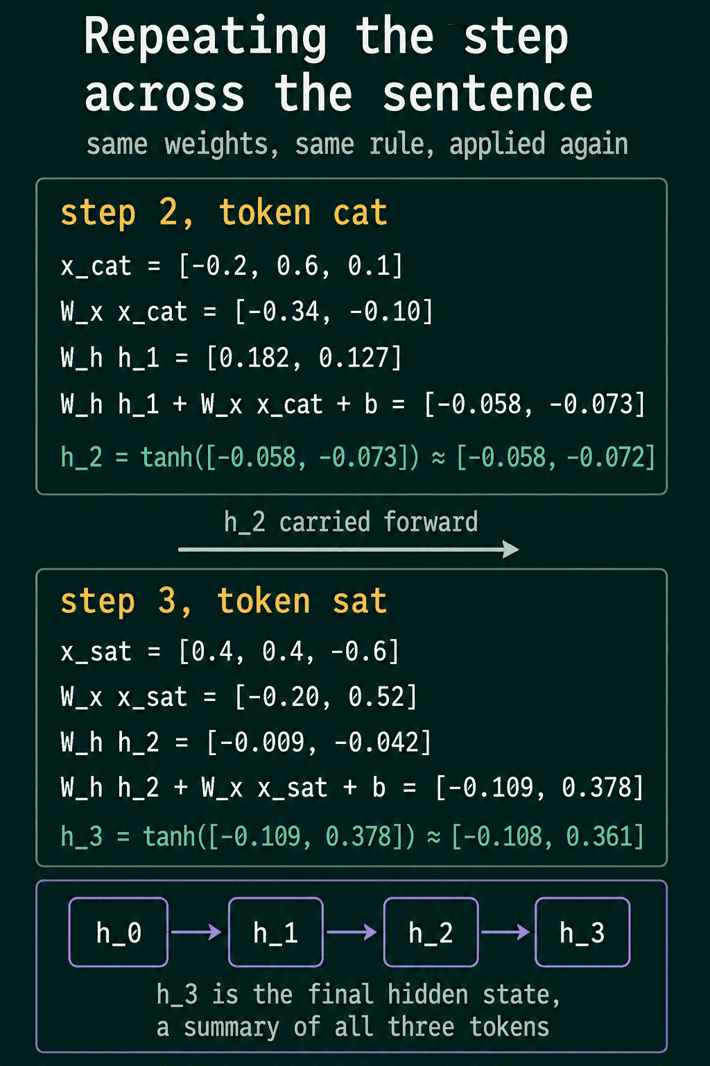

The second and third steps: for cat, W_x x_cat = [-0.34, -0.10] and W_h h_1 = [0.182, 0.127], giving h_2 about [-0.058, -0.072], and for sat, h_3 about [-0.108, 0.361], the final hidden state summarizing all three tokens.

Coding an RNN from scratch

In a model the update becomes a small module, called a cell, and a loop that applies it once per token. Each nn.Linear holds one weight matrix and its own bias, and the two biases add into the same sum before tanh:

1import torch
2import torch.nn as nn
3 
4class RNNCell(nn.Module):
5    def __init__(self, input_size, hidden_size):
6        super().__init__()
7        self.W_xh = nn.Linear(input_size, hidden_size)
8        self.W_hh = nn.Linear(hidden_size, hidden_size)
9 
10    def forward(self, x, h):
11        return torch.tanh(self.W_xh(x) + self.W_hh(h))
12 
13class RNN(nn.Module):
14    def __init__(self, input_size, hidden_size, num_classes):
15        super().__init__()
16        self.hidden_size = hidden_size
17        self.cell = RNNCell(input_size, hidden_size)
18        self.fc = nn.Linear(hidden_size, num_classes)
19 
20    def forward(self, x):
21        B, T, _ = x.shape
22        h = torch.zeros(B, self.hidden_size)
23        for t in range(T):
24            h = self.cell(x[:, t, :], h)
25        return self.fc(h)
26 
27model = RNN(input_size=3, hidden_size=2, num_classes=4)
28x = torch.randn(8, 5, 3)      # 8 sequences, 5 tokens each, 3 numbers per token
29print(model(x).shape)
30x = torch.randn(8, 50, 3)     # same model, 50 tokens
31print(model(x).shape)

1torch.Size([8, 4])
2torch.Size([8, 4])

x has shape (batch, seq_len, input_size), and x[:, t, :] picks the embeddings at position t for every sequence in the batch. The same model takes 5 tokens or 50 without any change, because the loop runs once per token with the same weights. self.fc reads only the final hidden state, which makes this version a classifier that gives one label per sequence.

Reading the hidden states: input and output modes

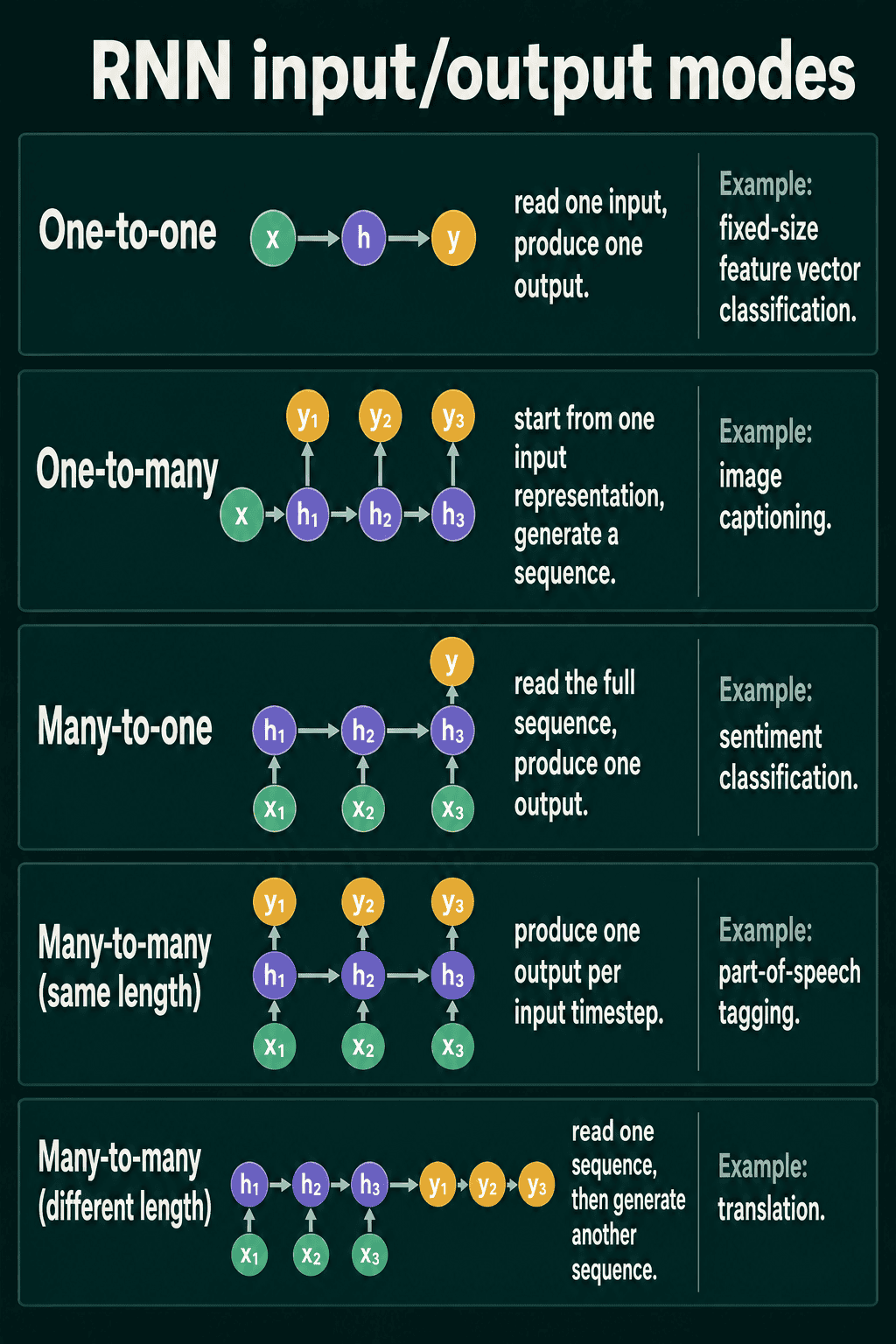
The loop produces a hidden state at every position, $\mathbf{h}_1, \mathbf{h}_2, \ldots, \mathbf{h}_T$, and different tasks read different ones. The small layer that turns the chosen hidden states into scores is called a head, and it is usually a linear layer from hidden_size to the number of things the task predicts. The common patterns are named by how many inputs the model reads and how many outputs it produces:

One-to-one: one input, one output, such as classifying one fixed-size feature vector.
One-to-many: one starting input, then a generated sequence, such as captioning an image by encoding it into the first hidden state and generating words.
Many-to-one: read the whole sequence and use the final hidden state $\mathbf{h}_T$, such as labelling a review positive or negative.
Many-to-many, same length: one output per input token from each $\mathbf{h}_t$, such as tagging every word with its part of speech.
Many-to-many, different length: one RNN reads the source sequence and a second RNN starts from its final state to generate the target, such as translation.

An RNN language model uses the same-length many-to-many pattern: the hidden state at each position goes through a head of size vocab_size to predict the next token.

The five RNN input and output modes, one-to-one, one-to-many, many-to-one, many-to-many with the same length and many-to-many with different lengths, each with an example task.

nn.RNN in PyTorch

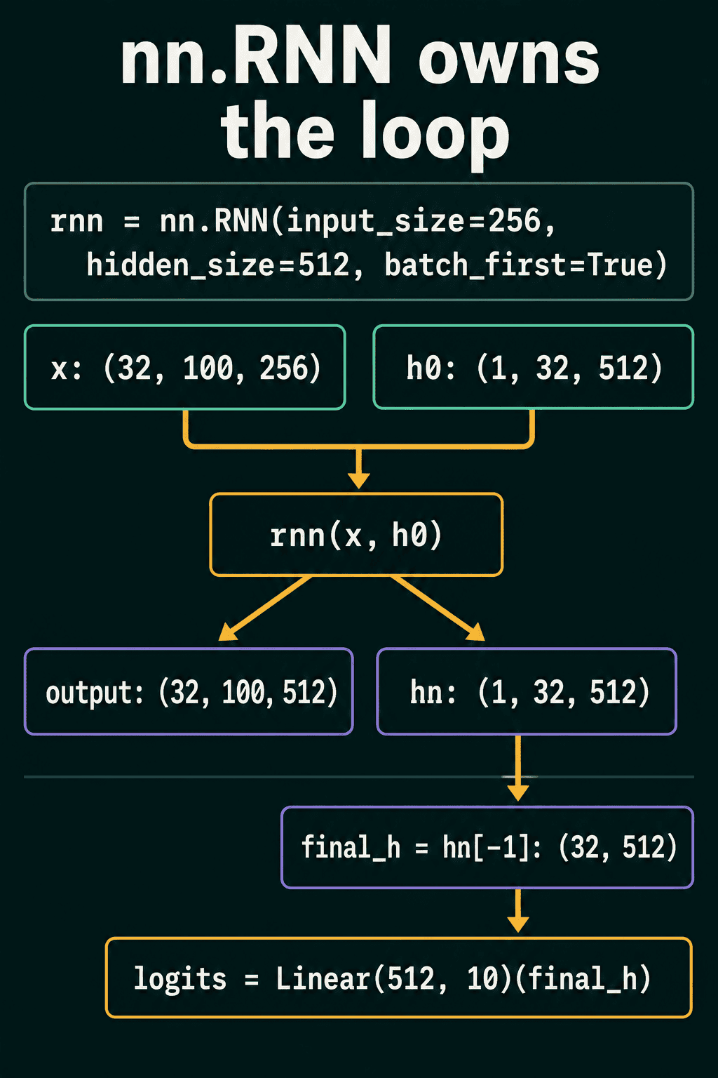
PyTorch has the loop built in as nn.RNN. It applies the same update at every position and returns two tensors. output holds the hidden state at every position, and hn holds the final hidden state:

1import torch
2import torch.nn as nn
3 
4rnn = nn.RNN(input_size=256, hidden_size=512, batch_first=True)
5 
6x = torch.randn(32, 100, 256)     # 32 sequences, 100 tokens, 256 numbers per token
7h0 = torch.zeros(1, 32, 512)
8 
9output, hn = rnn(x, h0)
10print(output.shape)   # one hidden state per token
11print(hn.shape)       # the final hidden state
12 
13vocab_head = nn.Linear(512, 1000)
14print(vocab_head(output).shape)          # next-token logits at every position
15class_head = nn.Linear(512, 10)
16print(class_head(hn[-1]).shape)          # one label for the whole sequence

1torch.Size([32, 100, 512])
2torch.Size([1, 32, 512])
3torch.Size([32, 100, 1000])
4torch.Size([32, 10])

batch_first=True makes the input shape (batch, seq_len, input_size). The extra leading 1 in h0 and hn counts layers, and hn[-1] takes the last one, giving shape (32, 512). A head on output makes one prediction per position, which is what a language model or a tagger needs. A head on hn[-1] makes one prediction per sequence.

nn.RNN with input_size 256 and hidden_size 512, x of shape (32, 100, 256) and h0 of shape (1, 32, 512) going in, output of shape (32, 100, 512) and hn of shape (1, 32, 512) coming out, and a linear head on hn[-1].

The fixed-size bottleneck

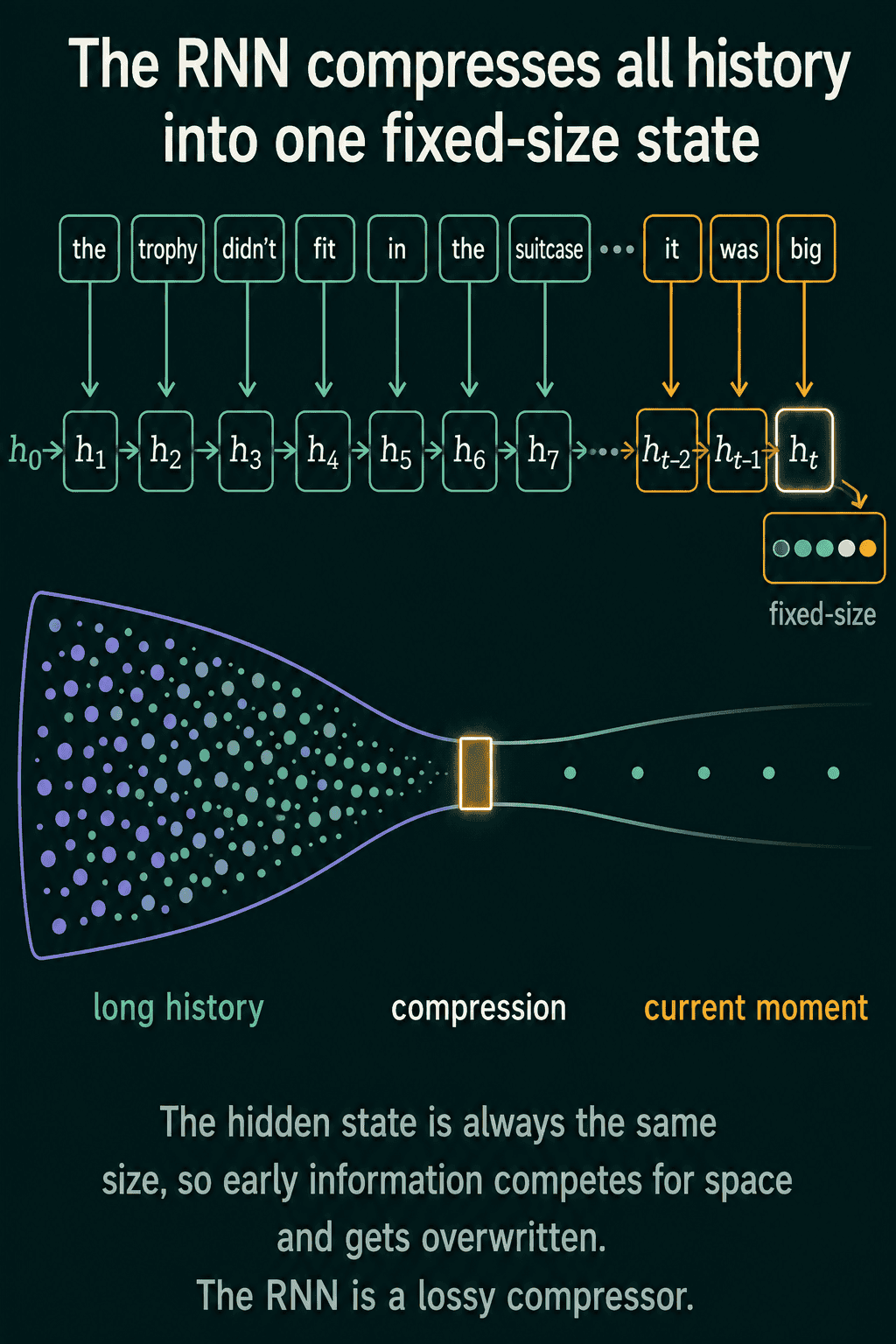
The hidden state is what makes an RNN work on sequences of any length, and it is also its main limit. It has the same size whether the sequence is 5 tokens or 500. Everything the model knows about the text so far has to fit in that one vector, and what goes into it is learned. As the sequence grows, older information competes for space with newer information, and details from early on can be overwritten before the model reaches the position that needs them.

The sentence the trophy didn't fit in the suitcase, it was big, read into hidden states h1 to h_t, with a long history narrowing into one fixed-size state.

How RNNs are trained: backpropagation through time

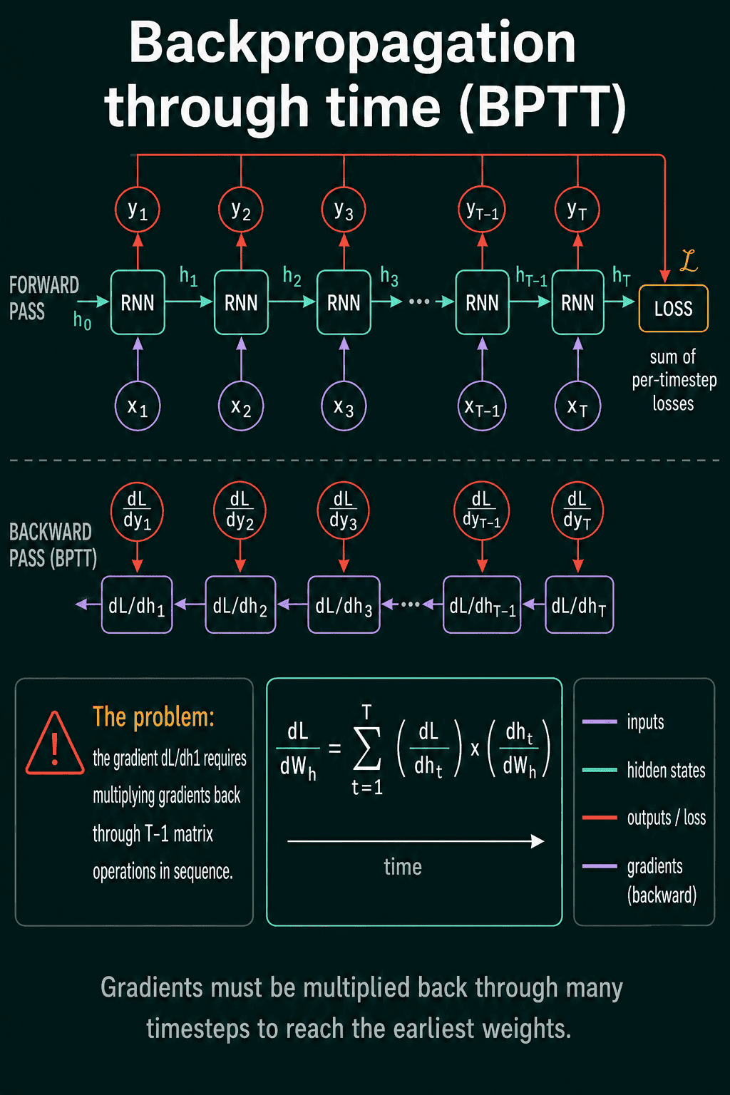
Training an RNN means computing the gradient of the loss with respect to $\mathbf{W}_h$, $\mathbf{W}_x$ and $\mathbf{b}$. The forward pass reuses the same cell at every time step. Training unrolls those repeated uses into one long chain of computations with one link per position. Ordinary backpropagation then runs backward along that chain. Running backpropagation through the unrolled sequence is called backpropagation through time, or BPTT.

For a sequence of $T = 100$ tokens, the forward pass computes $\mathbf{h}_1, \ldots, \mathbf{h}_{100}$ and the loss. The backward pass sends gradients through the same states in reverse order, from $\mathbf{h}_{100}$ back to $\mathbf{h}_1$. Because $\mathbf{W}_h$ is used at every step, its gradient is a sum of one contribution per step:

$$\frac{\partial \mathcal{L}}{\partial \mathbf{W}_h} = \sum_{t=1}^T \frac{\partial \mathcal{L}}{\partial \mathbf{h}_t} \cdot \frac{\partial \mathbf{h}_t}{\partial \mathbf{W}_h}$$

Here $\mathcal{L}$ is the loss, and each term is how much the loss changes through $\mathbf{W}_h$'s use at step $t$. PyTorch does all of this automatically: each call to the cell in the forward loop is recorded, and loss.backward() walks the record backward through every step.

Backpropagation through time: a forward pass through RNN cells producing outputs and a summed loss, and a backward pass sending gradients from dL/dh_T back to dL/dh_1.

Truncated BPTT

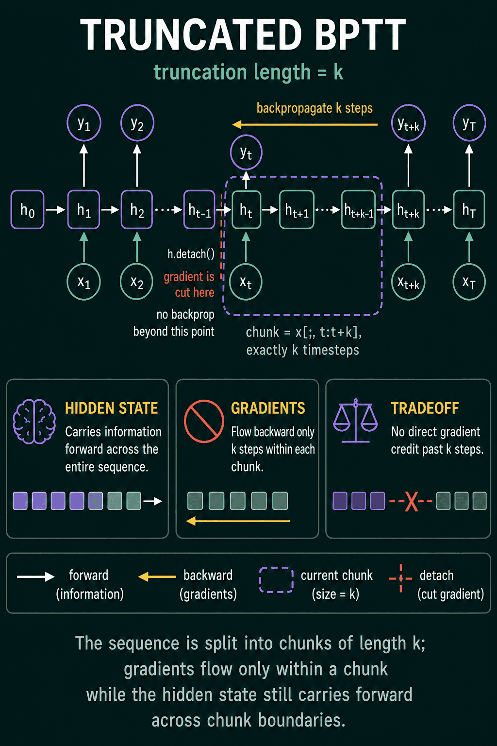
Full BPTT over $T = 1000$ steps has to keep the activations of all 1,000 steps in memory, and its backward pass grows with $T$. A common fix is truncated BPTT: split the sequence into chunks of $k$ steps and backpropagate only within each chunk.

1k = 50  # truncation length
2for t in range(0, T, k):
3    chunk = x[:, t:t+k]
4    h = h.detach()    # stop gradients from flowing back past this point
5    output, h = rnn(chunk, h)
6    loss = compute_loss(output)
7    optimizer.zero_grad()
8    loss.backward()
9    optimizer.step()

h.detach() keeps the value of the hidden state, so information still flows forward from one chunk to the next, but it cuts the gradient at the chunk boundary. The cost is that the model gets no direct gradient signal for dependencies longer than $k$ steps. Truncation also does not make the sequence faster to process, since step $t$ still needs step $t - 1$ first.

Truncated BPTT: the sequence split into chunks of length k, the hidden state carried forward across chunks, and gradients cut at each chunk boundary by h.detach().

Vanishing and exploding gradients

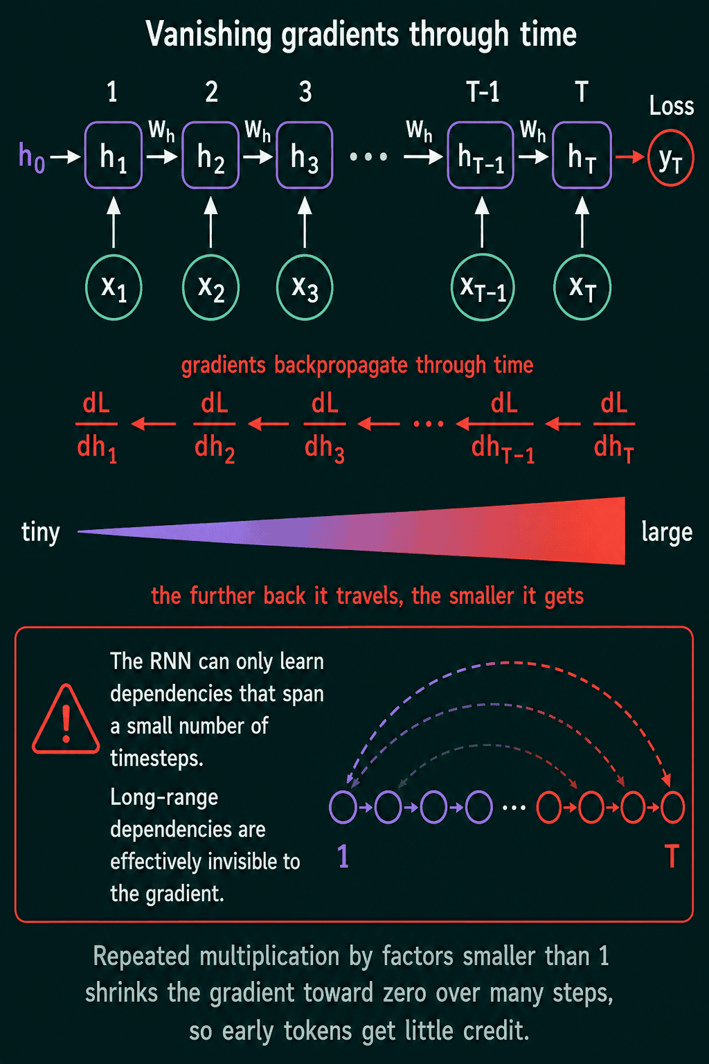
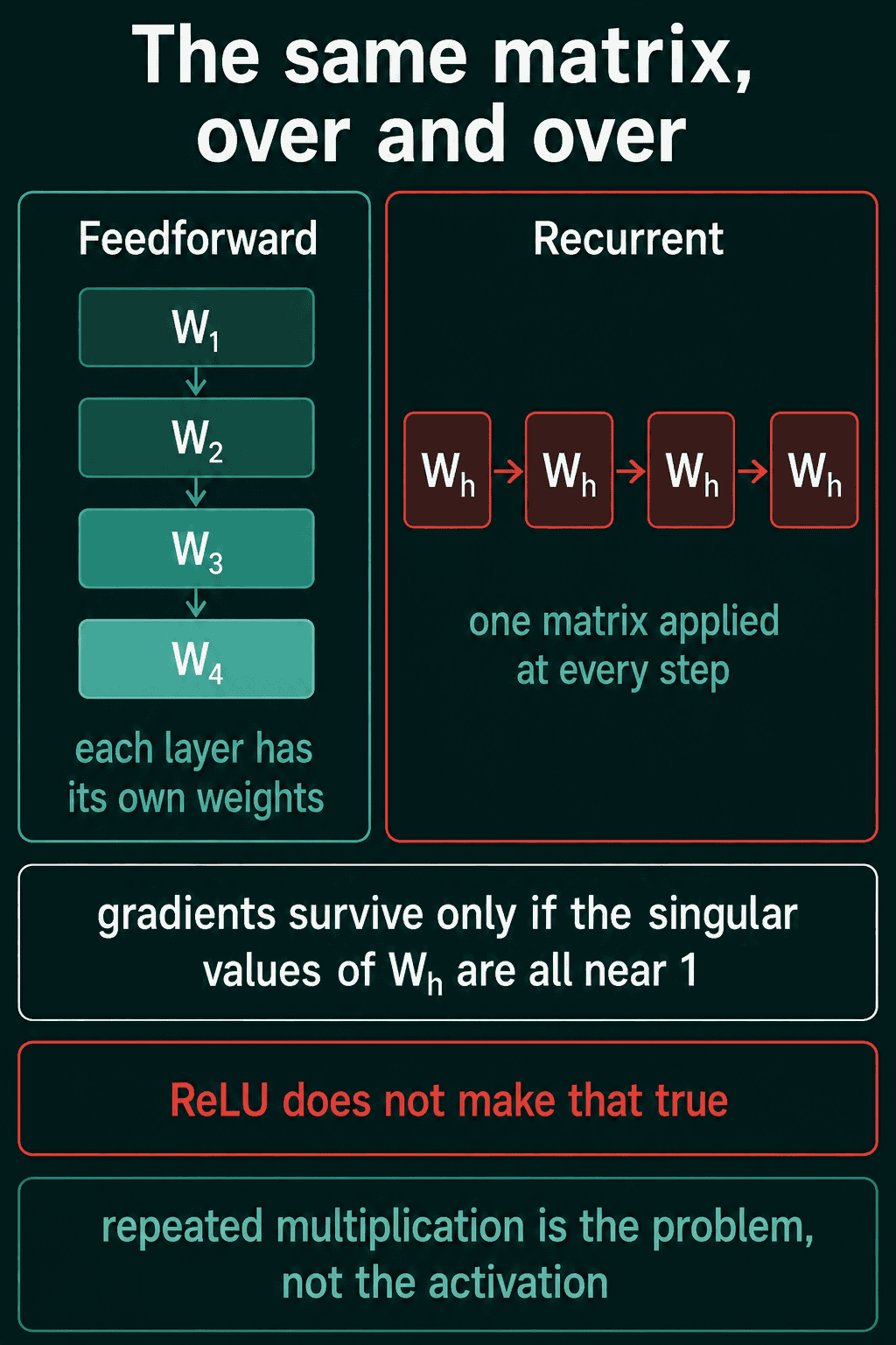
To reach $\mathbf{h}_1$, a gradient from the loss at step $T$ has to pass back through every step in between. At each step it gets multiplied by the same recurrent matrix (combined with the slope of tanh at that step), so over $T$ steps it is multiplied by nearly the same thing about $T - 1$ times:

$$\frac{\partial \mathbf{h}_T}{\partial \mathbf{h}_1} = \prod_{t=2}^{T} \frac{\partial \mathbf{h}_t}{\partial \mathbf{h}_{t-1}}$$

If each multiplication shrinks the gradient, the product decays toward 0. If each one grows it, the product blows up. Repeated multiplication does this fast, as a two-number gradient sent back 50 steps through a matrix that scales by 0.5 or by 1.5 shows:

1import torch
2 
3grad = torch.ones(2)
4for scale in [0.5, 1.5]:
5    W_h = scale * torch.eye(2)          # stretches every direction by the same amount
6    g = grad.clone()
7    for step in range(50):
8        g = W_h.T @ g                   # one step back through time
9    print(scale, f"{g.norm().item():.1e}")

10.5 1.3e-15
21.5 9.0e+08

Vanishing gradients are the first case. The gradient that reaches early steps is close to 0, so the model gets almost no signal for connecting a word to something many steps back, such as a pronoun to a noun 50 words earlier. The hidden state may still carry that information forward, but training cannot learn to use it.

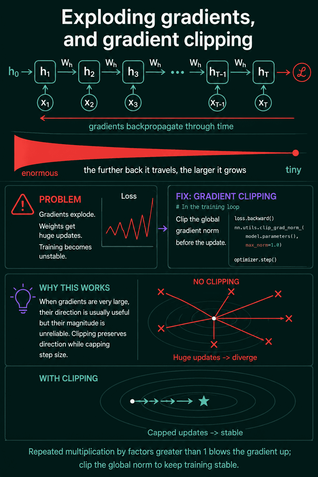
Gradients flowing back from the loss at step T to step 1 and shrinking from large to tiny, so the RNN learns only dependencies that span a few steps.

Exploding gradients are the second case. Huge gradients give the weights huge updates, and training becomes unstable: the loss spikes, jumps around or turns into nan. The usual fix is gradient clipping. Measure the length of the full gradient vector $\mathbf{g}$ across all parameters. If it is longer than a limit $c$, scale it down to length $c$:

$$\mathbf{g}_{\text{clipped}} = \mathbf{g} \cdot \min\left(1, \frac{c}{\lVert \mathbf{g} \rVert_2}\right)$$

The direction of a very large gradient is usually still useful, while its size is not. Clipping keeps the direction and caps the step. In PyTorch it goes between backward() and step():

1loss.backward()
2torch.nn.utils.clip_grad_norm_(model.parameters(), max_norm=1.0)
3optimizer.step()

Clipping is a common default when training RNNs.

Gradients growing as they travel back through time, the loss jumping around without clipping, and clip_grad_norm_ with max_norm=1.0 giving capped, stable updates.

Why ReLU does not fix it

In feedforward networks, switching from tanh to ReLU often reduces vanishing gradients, since ReLU's slope is 1 for positive inputs. In an RNN that change is not enough. A feedforward network has different weights in each layer, but an RNN multiplies by the same $\mathbf{W}_h$ at every step, so the size of that one matrix decides whether gradients shrink or grow. ReLU RNNs are more likely to explode, because ReLU has no upper limit on its output. The longer-term fix is a different cell design, such as the LSTM, which gives gradients a more direct path back through time.

A feedforward network with its own weights W1 to W4 per layer next to a recurrent network applying the same W_h at every step, with the note that ReLU does not change the singular values of W_h.

Bidirectional RNNs

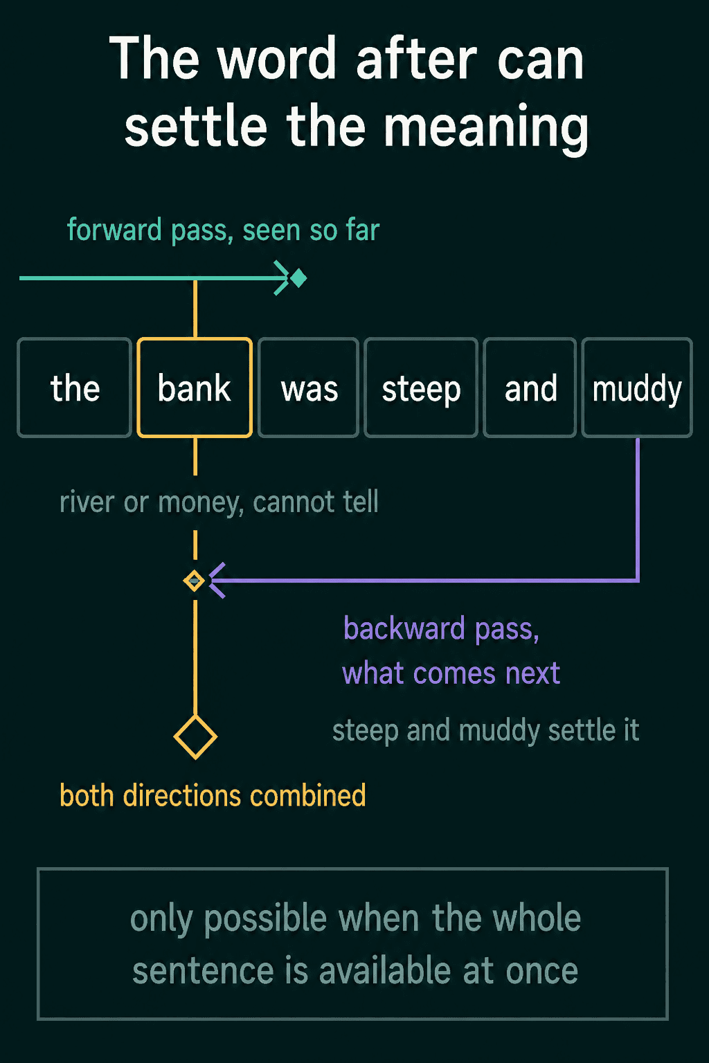
Sometimes the model is not writing the next word but labelling words in a sentence that already exists. To label bank in the bank was steep and muddy, the words before bank are not enough, since the bank could be about money. The words after it, steep and muddy, point to a river bank.

A bidirectional RNN runs two RNNs over the sentence, one left to right and one right to left. At each position it joins the two hidden states end to end. Call the forward state $\overrightarrow{\mathbf{h}}_t$ and the backward state $\overleftarrow{\mathbf{h}}_t$:

$$\mathbf{z}_t = [\overrightarrow{\mathbf{h}}_t, \overleftarrow{\mathbf{h}}_t]$$

If each direction has hidden size $H$, then $\mathbf{z}_t$ has size $2H$, and any layer that reads it has to expect the doubled width.

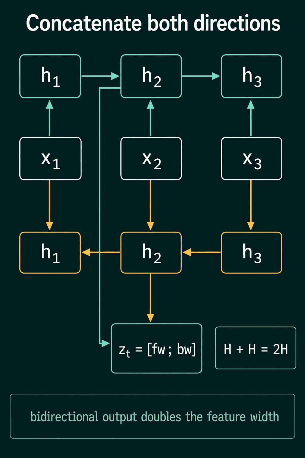
The sentence the bank was steep and muddy, with the forward pass reaching bank too early to decide river or money, and the backward pass bringing in steep and muddy.

A forward row and a backward row of hidden states over x1 to x3, with the two states at position 2 concatenated into z_t of width 2H.

In PyTorch it is one flag. output holds both directions side by side at every position, and for a single layer hn[-2] is the final forward state and hn[-1] the final backward state:

1import torch
2import torch.nn as nn
3 
4birnn = nn.RNN(input_size=16, hidden_size=32, batch_first=True, bidirectional=True)
5output, hn = birnn(torch.randn(4, 10, 16))
6print(output.shape)   # forward and backward states side by side
7print(hn.shape)       # final forward state, final backward state
8final = torch.cat([hn[-2], hn[-1]], dim=-1)
9print(final.shape)

1torch.Size([4, 10, 64])
2torch.Size([2, 4, 32])
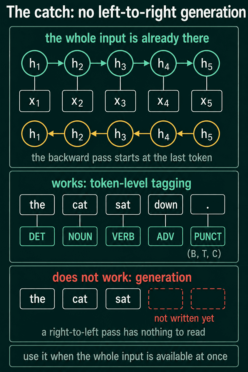
3torch.Size([4, 64])

A bidirectional RNN needs the whole input before it starts, because the backward pass begins at the last token. That fits tagging, named-entity recognition and sentence classification. It does not fit generating text left to right, since the tokens a backward pass would start from have not been written yet.

Bidirectional reading works for tagging the cat sat down with part-of-speech labels, and does not work for generation, where the next tokens are not written yet.

Stacked RNNs

One recurrent layer does everything with one hidden state per position. A stacked, or multi-layer, RNN feeds the hidden-state sequence of one layer into the next as its input. Layer 1 reads the token embeddings, layer 2 reads layer 1's hidden states, and so on. The time axis stays the same: each layer still has one vector per position, and each layer has its own weights.

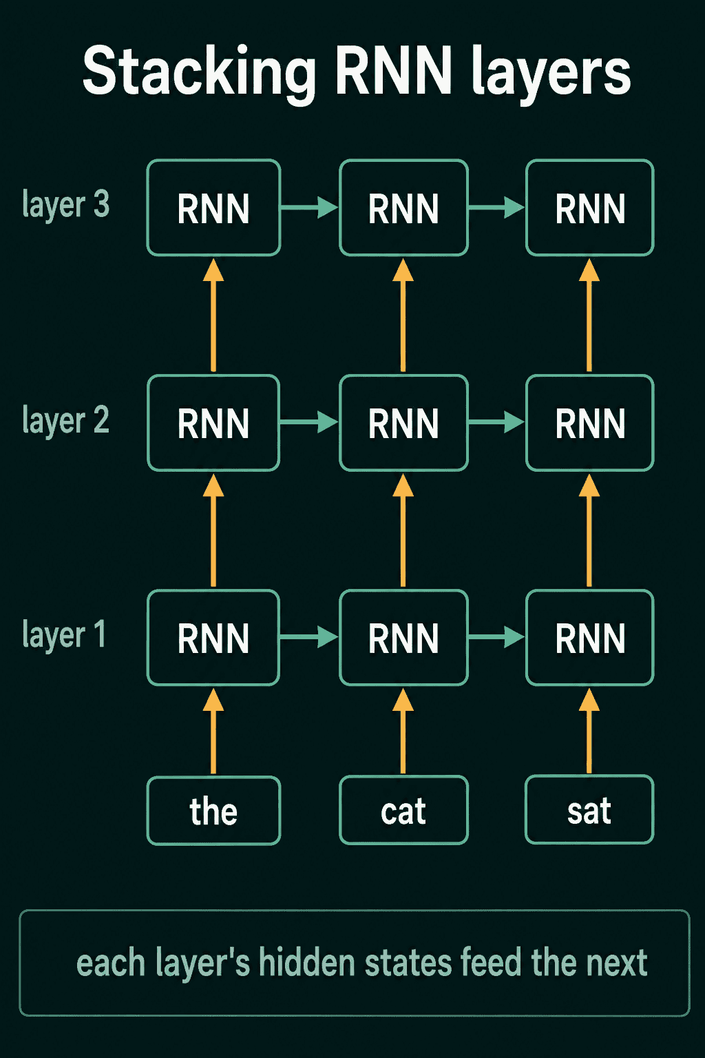
Three stacked RNN layers over the tokens the cat sat, each layer passing hidden states to the right and up into the layer above.

In PyTorch, num_layers sets the depth. output comes from the top layer at every position, and hn holds one final hidden state per layer:

1import torch
2import torch.nn as nn
3 
4stacked = nn.RNN(input_size=16, hidden_size=32, num_layers=3, batch_first=True, dropout=0.2)
5output, hn = stacked(torch.randn(4, 10, 16))
6print(output.shape)   # top layer, every position
7print(hn.shape)       # one final state per layer

1torch.Size([4, 10, 32])
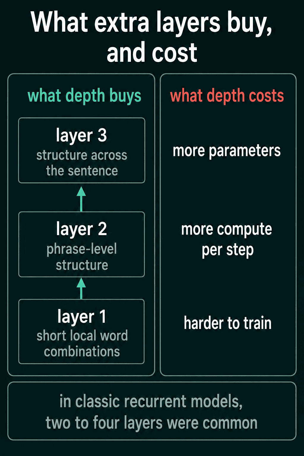
2torch.Size([3, 4, 32])

For classification, the head reads hn[-1], the top layer's final state. For tagging, it reads output. The dropout argument applies between stacked layers, so it does nothing when num_layers=1. Extra layers add parameters, memory and computation, and they can make training harder. In classic recurrent models two to four layers were common, and depth is usually chosen by checking results on validation data.

What extra layers add, more transformations at each position, and what they cost: more parameters, more computation per step and harder training.

Common mistakes

Reading hn for a tagging task. hn has one vector per sequence, so per-token predictions need output.
Forgetting the doubled width of a bidirectional RNN. The head after it needs 2 * hidden_size inputs.
Using a bidirectional layer in a text generator. The backward pass needs tokens that have not been generated yet.
Training without gradient clipping. One exploding batch can turn the loss into nan.
Forgetting h.detach() in truncated BPTT. Without it, gradients flow back through every earlier chunk, and memory grows with each chunk.
Expecting an RNN to use a token far back in a long sequence. Vanishing gradients make dependencies over many steps hard to learn.

The post on how language models are trained covers the next-token loss that an RNN language model is trained with, and the perplexity post covers how such a model is scored on test text. The LSTM and GRU are recurrent cells built to keep gradients from vanishing, and they use the same nn.LSTM and nn.GRU interface with bidirectional and num_layers. Transformers take a different route: every position can read every earlier position directly, instead of receiving information through one hidden state passed along one step at a time.

QuiddityML teaches RNNs in the language models unit of its NLP track, starting from the one-step update by hand. Its exercises include writing RNNCell and the loop from scratch, coding all five readout patterns with nn.RNN, and filling in a truncated BPTT training loop with h.detach() (QuiddityML).