4 October 2026 · 7 min read

Data leakage in machine learning: examples and how to prevent it

A model that scores well during development can still fail on new data when its evaluation was contaminated. This post shows common examples of data leakage, how to spot it on a loss curve, and how to prevent it in PyTorch.

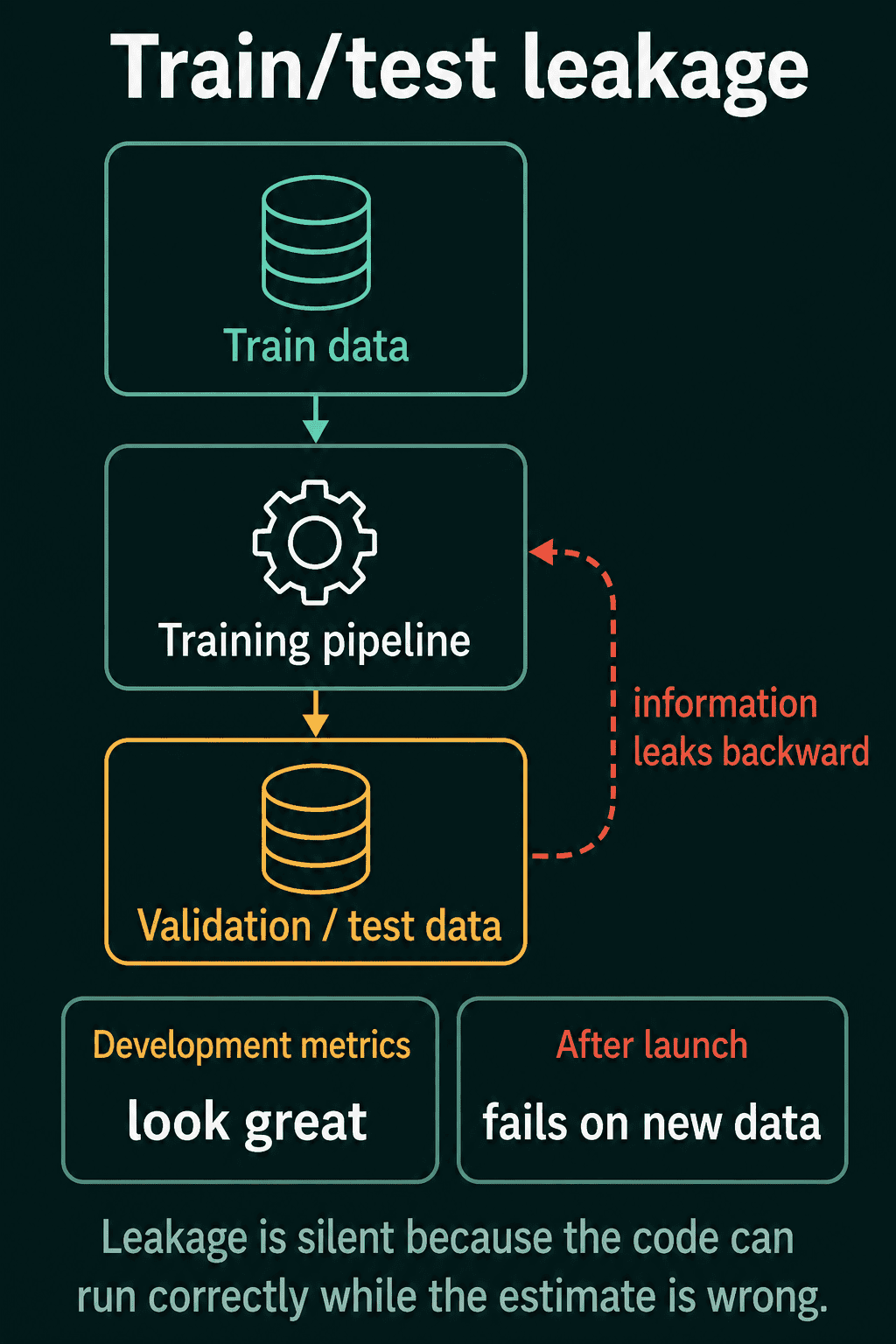
Data leakage is when information from the data a model is evaluated on reaches the model during training, even indirectly and even by accident. It makes the evaluation score look better than the model really is. Nothing crashes and the code runs fine, so a leaking model usually looks great during development and is found out when it meets real data after launch.

Why a score on your own data can mislead you

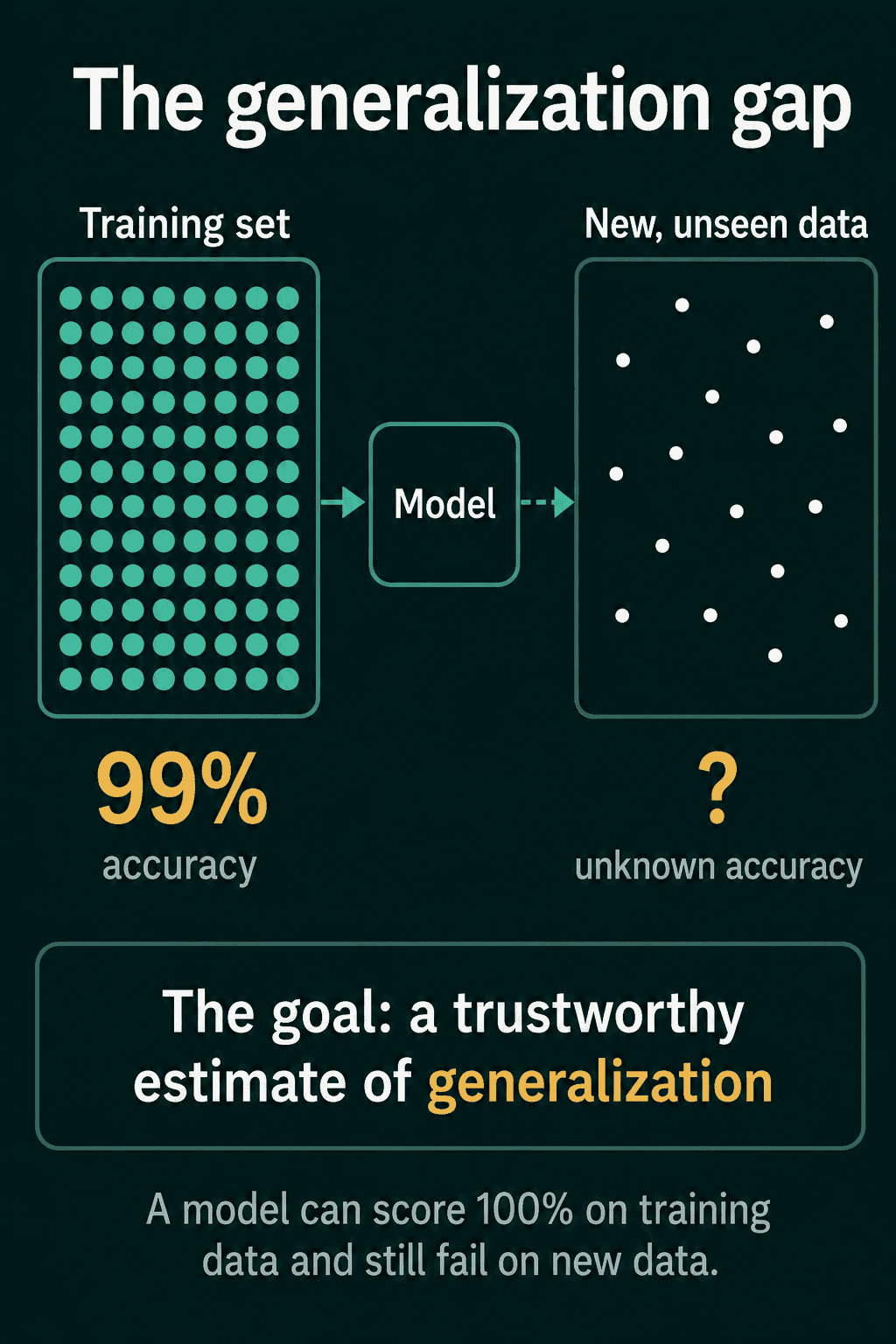
A model that scores 99% accuracy on the data it trained on may still be useless. A model that memorized its training examples would score close to 100% on them, so a high training score cannot tell memorizing apart from learning a pattern that carries over to new inputs.

What people actually want to know is generalization: how well the model does on data it did not train on. That data does not exist yet when the model is built, so the usual setup holds some of the available data back:

the training set is what the model learns its weights from
the validation set is used to make choices, such as the learning rate or when to stop training
the test set is scored once at the end, as the estimate of performance on new data

The held-out sets stand in for future data, and that works as long as nothing from them reaches the model while it trains. The train, validation, and test split post covers making the split.

A model scores 99% accuracy on its training set while its accuracy on new, unseen data is unknown, and the goal is a trustworthy estimate of generalization

What data leakage is

Leakage happens when the validation or test set influences any part of the training pipeline: the preprocessing, the choice of features, or the training rows themselves. During development, the leaked information is present in both the training pipeline and the evaluation, so the metrics look excellent. After launch the model sees data that played no part in training, the advantage disappears, and performance drops to what the model can really do.

Train data flows into the training pipeline, which is evaluated on validation and test data, while a dashed red arrow shows information leaking backward from the validation and test data into the pipeline, so development metrics look great and the model fails on new data after launch

Common examples of data leakage

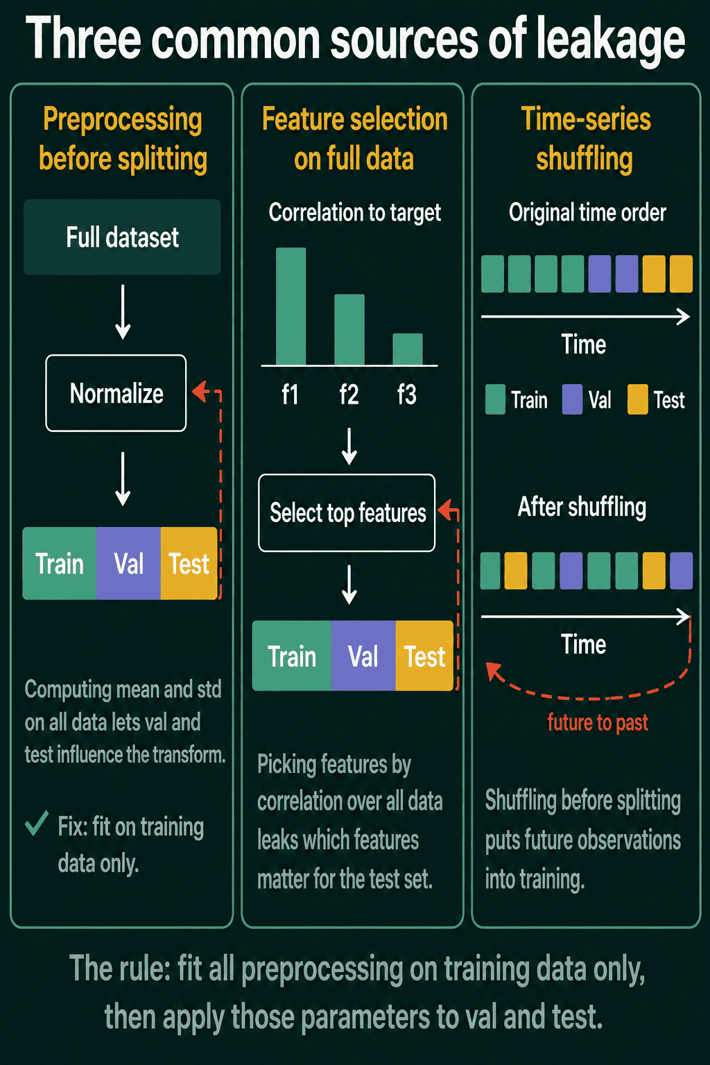
1. Preprocessing fitted on the full dataset. Normalization rescales each input feature so it has mean 0 and standard deviation 1. For a feature value $x$, with $\mu$ the mean of that feature and $\sigma$ its standard deviation:

$$x' = \frac{x - \mu}{\sigma}$$

$x'$ is how many standard deviations $x$ sits from the mean. The leak is in where $\mu$ and $\sigma$ come from. If they are computed on the whole dataset before splitting, the validation and test rows helped set them, and the transform the model trains with already carries information about those rows.

2. Feature selection on the full dataset. A common way to pick features is to keep the ones most correlated with the label. If that correlation is computed over the full dataset, test rows included, the selection step has looked at the test labels and kept the features that happen to line up with them.

3. Shuffling a time series before splitting. With data ordered in time, such as daily sales, a random shuffle puts later observations into the training set and earlier ones into the test set. The model then trains on the future and is graded on predicting the past, which it will not get to do in production.

Three panels: normalizing before the split lets validation and test data influence the transform, selecting features by correlation over the full data leaks which features line up with the test labels, and shuffling a time series puts future observations into training

Data leakage in code

The first snippet uses 1,000 sensor readings in time order, where the last 200 come from a later period with higher readings. It normalizes the test rows two ways:

1import torch
2 
3torch.manual_seed(0)
4# 1,000 sensor readings in time order, the last 200 from a later period when readings ran higher
5readings = torch.cat([torch.randn(800) + 10.0, torch.randn(200) + 13.0])
6train, test = readings[:800], readings[800:]
7 
8mean_all, std_all = readings.mean(), readings.std()   # leaky: computed before the split
9mean_tr, std_tr = train.mean(), train.std()           # correct: computed on the 800 train rows
10 
11print(f"1,000 rows:  mean {mean_all:.2f}, std {std_all:.2f}")
12print(f"train rows:  mean {mean_tr:.2f}, std {std_tr:.2f}")
13print(f"test mean after leaky scaling: {((test - mean_all) / std_all).mean():.2f}")
14print(f"test mean after train scaling: {((test - mean_tr) / std_tr).mean():.2f}")

11,000 rows:  mean 10.63, std 1.53
2train rows:  mean 10.07, std 1.02
3test mean after leaky scaling: 1.48
4test mean after train scaling: 2.76

With statistics from the 800 training rows, the test readings sit 2.76 standard deviations above the training data. The leaky statistics pulled the mean toward the test rows and widened the standard deviation, so the same shift shows up as 1.48.

The second snippet shows the feature selection leak. It builds 2,000 features of random noise and coin-flip labels, so no model can do better than 50% on new data:

1import torch
2import torch.nn.functional as F
3 
4torch.manual_seed(0)
5X = torch.randn(300, 2000)                 # 300 rows, 2,000 features of pure noise
6y = torch.randint(0, 2, (300,)).float()    # labels are coin flips, so 50% is the real ceiling
7train, test = torch.arange(200), torch.arange(200, 300)
8 
9def top_features(X, y, k=20):
10    """Indices of the k features most correlated with the label."""
11    Xc, yc = X - X.mean(0), y - y.mean()
12    corr = (Xc * yc[:, None]).sum(0) / (Xc.norm(dim=0) * yc.norm())
13    return corr.abs().topk(k).indices
14 
15def test_accuracy(cols):
16    """Train logistic regression on the train rows, score it on the test rows."""
17    w = torch.zeros(len(cols), requires_grad=True)
18    b = torch.zeros(1, requires_grad=True)
19    opt = torch.optim.SGD([w, b], lr=0.1)
20    for _ in range(500):
21        opt.zero_grad()
22        F.binary_cross_entropy_with_logits(X[train][:, cols] @ w + b, y[train]).backward()
23        opt.step()
24    pred = (X[test][:, cols] @ w + b > 0).float()
25    return (pred == y[test]).float().mean().item()
26 
27print(f"features picked on 300 rows:       test accuracy {test_accuracy(top_features(X, y)):.2f}")
28print(f"features picked on 200 train rows: test accuracy {test_accuracy(top_features(X[train], y[train])):.2f}")

1features picked on 300 rows:       test accuracy 0.68
2features picked on 200 train rows: test accuracy 0.52

The model trains on the same 200 rows both times. When the 20 features were chosen with the test labels in view, it scores 68% on labels that are pure chance. Chosen from the training rows, it scores 52%, close to the 50% it should get. If a result like the first line shows up in a real project, the first thing to check is whether any step before training saw rows outside the training set.

Validation contamination

Even with no bug in the pipeline, the validation score drifts upward over a project. Each time the validation score decides something, such as the learning rate, the number of layers, or the epoch to stop at, the chosen settings fit that particular validation set a little better.

Run 50 hyperparameter configurations, each one a trial with its own validation accuracy, and keep the one with the highest score. The best validation score so far rises or stays flat as trials are added, because a new trial replaces the leader whenever it beats it. That winning score is optimistic: part of why it won is luck on this specific split, so the winner's true performance on unseen data sits below it. The distance between the two is the selection gap.

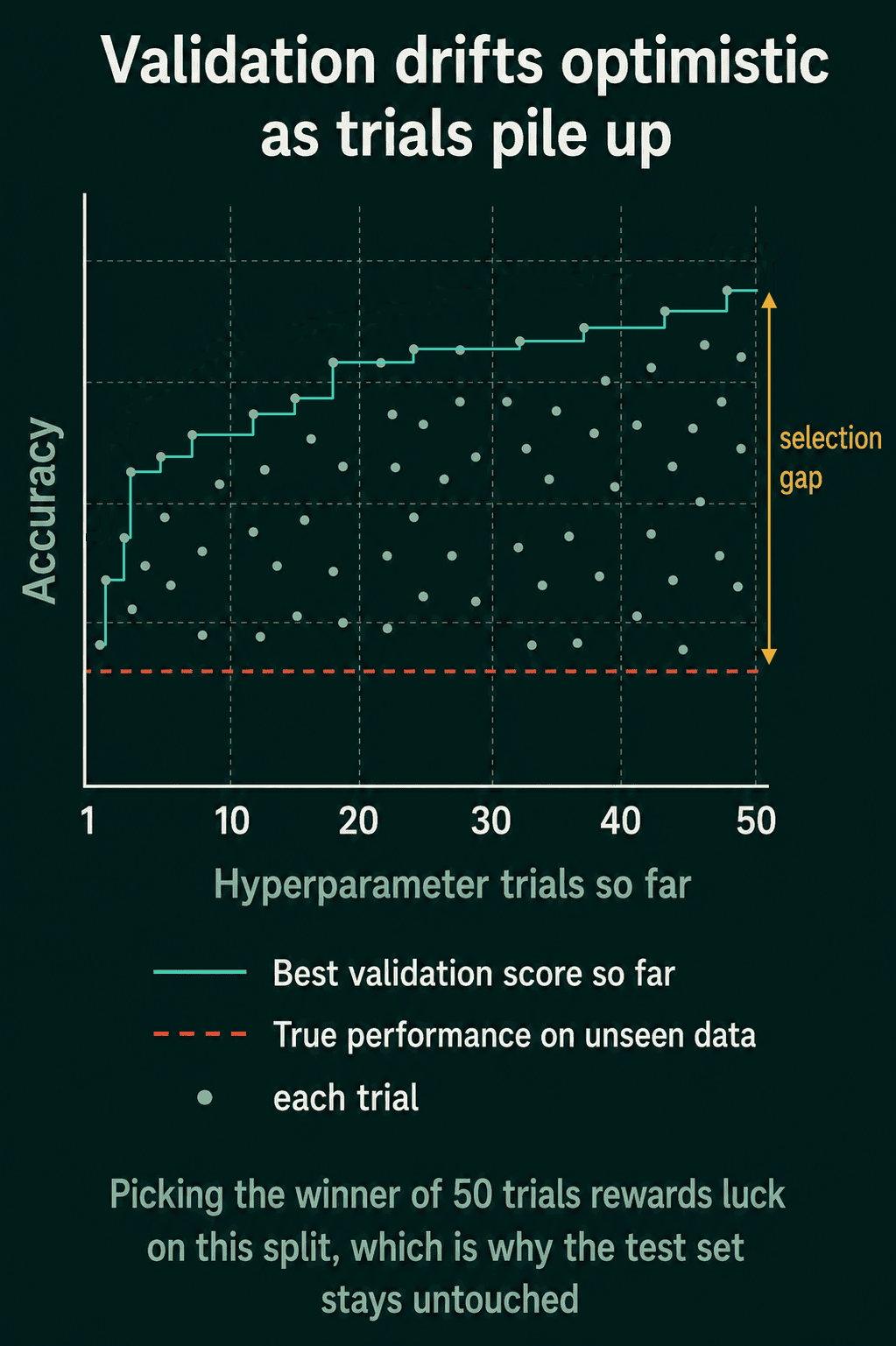
Each of 50 hyperparameter trials is a dot, the best validation score so far steps upward through the highest dots, and a selection gap separates it from the lower, flat true performance on unseen data

This is normal and is what hyperparameter search does, covered in grid vs random search. It is also why the test set stays out of model and hyperparameter decisions. The validation score is for choosing between models, and the test score is the clean final estimate.

How to spot leakage on a loss curve

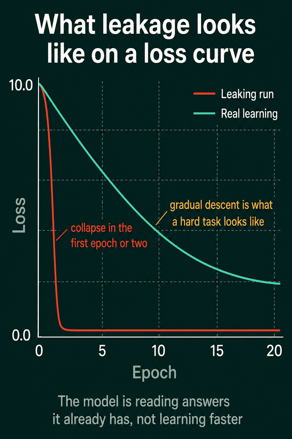
On a hard task, real learning shows up as a gradual drop in loss over many epochs. Leakage often looks different: the loss falls to near zero in the first epoch or two, much faster than the problem should allow. The model is reading answers it already has, through a feature that encodes the target or through validation rows that also sit in the training set. The loss curve post covers the other shapes a curve can take.

How to prevent data leakage

Fit preprocessing on the training rows. Compute the mean and standard deviation from the training set, then apply those same numbers to validation and test.
Select features on the training rows. Rank features by their correlation with the label using training data, then keep that same set for validation and test.
Keep a time series in time order. Do not shuffle it before splitting, so no future observations end up in training.
Leave the test set untouched while making decisions, and score it at the end as the clean final estimate.

A common mistake is celebrating a loss that drops to near zero in the first epoch or two instead of checking the pipeline first.

Cross-validation scores a model on several different splits of the same data instead of one. Metrics such as precision, recall, and F1 and ROC AUC are other ways to score a model on the validation or test set, and a leak inflates them the same way it inflates accuracy.

QuiddityML teaches leakage across three concepts in the ML Foundation track, and the exercises on them ask what leaks when a scaler is fitted before the split, what goes wrong when a time series is shuffled before an 80/20 split, and what a loss that collapses to near zero within two epochs points to.