28 September 2026 · 6 min read

The universal approximation theorem explained (and what it does not promise)

The universal approximation theorem says a neural network with one wide enough hidden layer can match any continuous curve as closely as you like. This post explains what that means, why it works, and the four things the theorem does not promise about training and real data.

The universal approximation theorem says that a neural network with a single hidden layer, a suitable activation function, and enough neurons can match any continuous function on a bounded range of inputs as closely as you want. It is the usual answer to the question "why should a neural network be able to learn this at all?", and it says much less about training than it is often taken to say.

What a hidden layer is

A neural network takes an input, such as a number $x$, and produces an output. In between sit hidden layers: groups of neurons whose outputs are not the final answer but are passed on to the next layer. A single neuron multiplies its input by a weight, adds a bias (one extra learned number), and passes the result through an activation function, a small fixed function like $\tanh$ or ReLU that bends the straight line into a curve. ReLU outputs its input when it is positive and 0 otherwise.

A network with one hidden layer of $N$ neurons does this $N$ times in parallel, with $N$ different weights and biases, then adds up the $N$ results, each multiplied by its own output weight. $N$ is called the width of the layer. The weights and biases are the network's parameters, the numbers training adjusts.

The problem the theorem answers

A model can only learn patterns it is able to represent. A straight line $y = wx + b$ cannot fit a curve no matter how it is trained, because no choice of $w$ and $b$ bends it. So before training a network on a messy relationship between inputs and outputs, it is fair to ask whether any setting of its weights could produce that relationship.

For a network with one hidden layer, the answer is yes, under three conditions:

The target function is continuous: it has no jumps.
The inputs stay inside a bounded region, such as $x$ between -2 and 2. The formal term is a compact set, meaning closed and bounded.
The activation function is non-polynomial. Sigmoid, $\tanh$ and ReLU all qualify. A network with no activation at all does not, because stacking linear layers produces another linear function.

If those hold, then for any error tolerance you pick, some finite width $N$ gets the network within that tolerance everywhere in the region. That statement is the universal approximation theorem.

The idea behind it

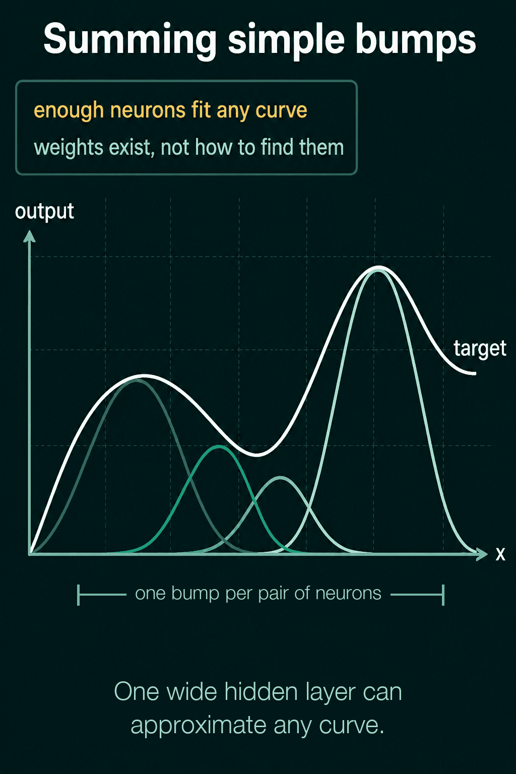
Each hidden neuron produces a response that is large for some inputs and small for others. With $\tanh$, one neuron gives a smooth step up at a position set by its weight and bias. Two neurons whose steps are placed close together and subtracted give a bump: near zero on both sides, high in between. A bump's height is set by its output weight.

Place enough bumps along the input range, each scaled to the height of the target curve at that spot, and their sum traces the curve. Narrower bumps follow the curve more closely, and more of them are needed to cover the range, which is where the width comes from.

A wavy target curve on x and output axes, with four overlapping teal bumps underneath whose peaks touch the curve at different points, labeled one bump per pair of neurons, with a note that weights to fit the curve exist but the theorem does not say how to find them.

The statement in math

Write the input as a vector $x$ with $d$ numbers, the target function as $f$, and the bounded region as $K$. Hidden neuron $i$ has weights $w_i$ (a vector of $d$ numbers), a bias $b_i$, and an output weight $v_i$. The activation function is $\varphi$. The network's output is the sum over its $N$ neurons of $v_i , \varphi(w_i^\top x + b_i)$, where $w_i^\top x$ is the dot product of $w_i$ and $x$.

The theorem says that for any tolerance $\varepsilon > 0$, there is a width $N$ and a choice of all these numbers such that

$$\sup_{x \in K} \left| f(x) - \sum_{i=1}^{N} v_i,\varphi(w_i^{\top}x + b_i) \right| < \varepsilon$$

$\sup_{x \in K}$ means "the largest value over all inputs in $K$", so the equation says the worst-case gap between the target and the network, anywhere in the region, is smaller than $\varepsilon$. In PyTorch that sum is the shape of nn.Sequential(nn.Linear(d, N), nn.Tanh(), nn.Linear(N, 1)).

Testing it in PyTorch

This snippet fits $f(x) = \sin(3x) + 0.3x^2$ on $x$ between -2 and 2 with one-hidden-layer networks of different widths, trained with the Adam optimizer. It also measures the error on $x$ between 3 and 4, a range the network never saw.

1import torch
2import torch.nn as nn
3 
4torch.manual_seed(0)
5 
6def target(x):
7    return torch.sin(3 * x) + 0.3 * x ** 2
8 
9x_train = torch.linspace(-2, 2, 400).unsqueeze(1)   # shape (400, 1)
10y_train = target(x_train)
11x_outside = torch.linspace(3, 4, 100).unsqueeze(1)  # outside the training range
12y_outside = target(x_outside)
13 
14def fit(width, steps=3000, lr=0.01):
15    model = nn.Sequential(nn.Linear(1, width), nn.Tanh(), nn.Linear(width, 1))
16    opt = torch.optim.Adam(model.parameters(), lr=lr)
17    loss_fn = nn.MSELoss()
18    for _ in range(steps):
19        opt.zero_grad()
20        loss = loss_fn(model(x_train), y_train)
21        loss.backward()
22        opt.step()
23    with torch.no_grad():
24        inside = loss_fn(model(x_train), y_train).item()
25        outside = loss_fn(model(x_outside), y_outside).item()
26    return inside, outside
27 
28for width in [1, 2, 4, 16, 64]:
29    inside, outside = fit(width)
30    print(f"width {width:>3}: MSE on [-2, 2] = {inside:.5f}, MSE on [3, 4] = {outside:.2f}")

On one CPU run, it printed:

Width	MSE on [-2, 2]	MSE on [3, 4]
1	0.30302	9.42
2	0.11297	7.44
4	0.00230	0.42
16	0.00001	0.15
64	0.00006	4.25

MSE (mean squared error) is the average squared gap between the network's output and the target. Inside the training range, going from 1 to 16 neurons takes the error from 0.3 to about 0.00001, so training reached the kind of close fit the theorem says exists. Two other things show up in the same table. The 64-neuron network can represent everything the 16-neuron one can, yet training left it with a higher error, and outside the range the error is 30 to over 10,000 times larger than inside and jumps around from width to width. Your exact numbers may differ on other hardware or PyTorch versions. If a width that should fit leaves a high error inside the range, change the learning rate or the number of steps first.

What the theorem does not promise

The theorem guarantees that good weights exist. It is silent on four things people often read into it:

How wide "enough" is. The width it guarantees can be enormous. For functions with many wiggles, or inputs with many dimensions, the neuron count a single hidden layer needs can grow far past anything practical.
Whether training finds the weights. Gradient descent adjusts weights step by step to lower the error, and it can stop at weights that fit worse than the best ones available, as the 64-neuron run above shows. Being able to represent a function is expressiveness. Reaching it by training is trainability, and the theorem covers only the first.
What happens outside the region. The guarantee holds on the bounded region $K$ and nowhere else. The network's output on $x$ between 3 and 4 in the run above is whatever the fitted neurons happen to produce there.
Whether the model generalizes. Real training data is a finite set of noisy samples, not the full function. A network wide enough to match any curve can also match the noise, and doing well on new data is a separate question the theorem does not touch.

It also does not say that one wide hidden layer is the architecture to use. Deeper networks often reach a given accuracy with fewer parameters, which is why most practical networks stack many layers.

Common mistakes

Treating the theorem as a reason any network will learn any task. When a network fails to fit, the theorem rules out nothing: the width might be too small, the optimizer might be stuck, or the data might not contain the pattern.
Forgetting the activation. Two nn.Linear layers with nothing between them collapse into one linear layer, and no width fixes that.
Trusting a fit outside the training range. A network that matches the data closely between -2 and 2 can be far off at 3.

The multilayer perceptron is the network the theorem is about: layers of neurons with activations between them. Activation functions are the non-polynomial piece the theorem needs, and the activation functions roadmap compares the common ones. Depth is the practical alternative to one enormous layer, since each layer can build on patterns found by the layer before it. Overfitting is the generalization gap in the last bullet above, a model fitting its training data closely and new data badly.

QuiddityML teaches the universal approximation theorem as its own concept in Unit 2 of the ML Foundation track, with multiple-choice questions on what the theorem guarantees and what it leaves open, and an exercise that matches its equation to the one-hidden-layer nn.Sequential it describes (quiddityml.com).