28 September 2026 · 8 min read

What is a neural network? The multilayer perceptron explained

A neural network passes its input through layers of simple units, each layer reshaping the numbers for the next one. This post explains the multilayer perceptron layer by layer, why stacking layers helps, and how to count its parameters by hand and in PyTorch.

A neural network is a model made of layers of small units called neurons, where each layer takes a list of numbers, transforms it, and hands the result to the next layer until the last layer produces a prediction. The multilayer perceptron (MLP) is the plainest version of this design, and it shows up inside larger models too: the feed-forward block in a transformer, for example, is a small MLP.

Why one neuron is not enough

A single artificial neuron takes some input numbers, multiplies each one by its own weight, adds the products together, and adds one more number called the bias. The weights and bias are the neuron's parameters, the numbers that training adjusts.

That calculation can only split its inputs with a straight line (or a flat plane, with more inputs). Some simple problems cannot be solved that way. The classic one is XOR: with two inputs that are each 0 or 1, the answer is 1 when exactly one input is 1. The two 1-cases sit on one diagonal of a square and the two 0-cases on the other, and no single straight line puts them on opposite sides. The perceptron post works through that limit in detail.

To get past it, a model needs several transformations in a row, where each one works on the output of the one before.

Input, hidden, and output layers

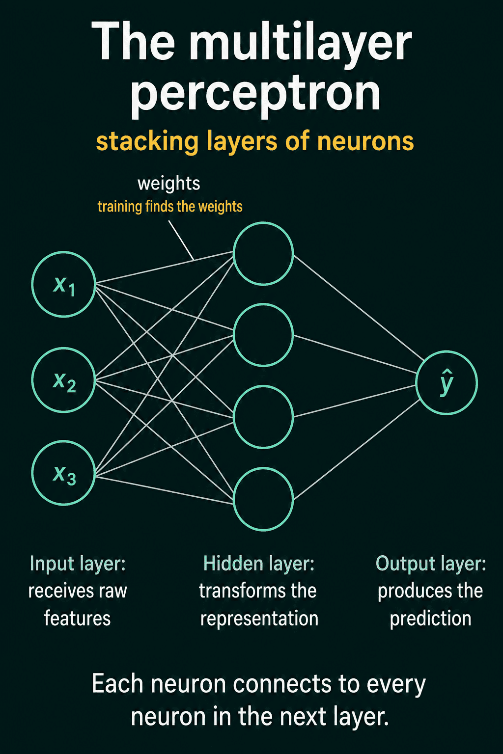
A multilayer perceptron stacks neurons into layers:

Input layer: holds the raw features, such as the pixel values of an image or the columns of a spreadsheet row. It does no computation.
Hidden layers: each one transforms the numbers it receives into a new list of numbers.
Output layer: produces the final prediction.

Each neuron in one layer connects to every neuron in the next layer, which is why these are also called fully connected layers. Every connection has its own weight, and training finds the values of all of them.

A multilayer perceptron with 3 inputs, a hidden layer of 4 neurons, and 1 output, where every input connects to every hidden neuron and every hidden neuron connects to the output.

The math of a one-hidden-layer MLP

Writing each layer as one matrix calculation keeps the math short. The pieces:

$\mathbf{x}$ is the input, a vector (list) of $d_{\text{in}}$ numbers.
$\mathbf{W}1$ is the first layer's weight matrix, with $d_h$ rows and $d{\text{in}}$ columns, where $d_h$ is the number of hidden neurons. Row $i$ holds the weights of hidden neuron $i$.
$\mathbf{b}_1$ is a vector of $d_h$ biases, one per hidden neuron.
$f$ is the activation function, a nonlinear function applied to each number separately. A common default is ReLU, $\mathrm{ReLU}(z) = \max(0, z)$, which keeps positive numbers and turns negative ones into 0.
$\mathbf{W}_2$ and $\mathbf{b}_2$ are the output layer's weights and biases.

The forward pass, the calculation that turns an input into a prediction, is two lines:

$$\mathbf{h} = f(\mathbf{W}_1 \mathbf{x} + \mathbf{b}_1)$$

$$\hat{y} = \mathbf{W}_2 \mathbf{h} + \mathbf{b}_2$$

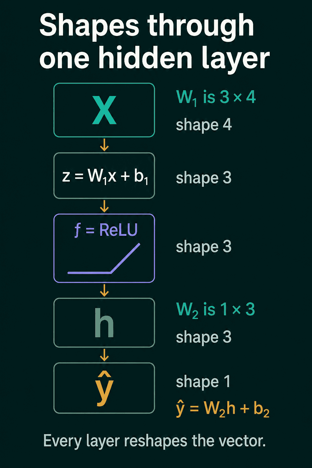
The first line computes every hidden neuron's weighted sum at once, $\mathbf{z} = \mathbf{W}_1 \mathbf{x} + \mathbf{b}_1$, and passes it through $f$ to get $\mathbf{h}$. The second line treats $\mathbf{h}$ as the input to one more weighted sum, which gives the prediction $\hat{y}$ (read "y hat"). A network with more hidden layers repeats the first line once per layer.

Take an input with 4 features, 3 hidden neurons, and 1 output. $\mathbf{W}_1$ is $3 \times 4$, so the 4 inputs become 3 numbers. ReLU keeps that length at 3. $\mathbf{W}_2$ is $1 \times 3$, so the 3 hidden numbers become one prediction.

The shapes through one hidden layer: an input x of length 4, multiplied by a 3 by 4 matrix W1 plus b1 to give z of length 3, ReLU keeping length 3 to give h, then a 1 by 3 matrix W2 plus b2 giving a single output y hat.

Why the activation function is needed

Without $f$, the hidden layer adds nothing. Plug the first line into the second:

$$\hat{y} = \mathbf{W}_2(\mathbf{W}_1 \mathbf{x} + \mathbf{b}_1) + \mathbf{b}_2$$

$$= (\mathbf{W}_2 \mathbf{W}_1)\mathbf{x} + (\mathbf{W}_2 \mathbf{b}_1 + \mathbf{b}_2)$$

$\mathbf{W}_2 \mathbf{W}_1$ is one matrix and $\mathbf{W}_2 \mathbf{b}_1 + \mathbf{b}_2$ is one vector, so the two layers compute exactly what a single layer could. The same algebra collapses any number of stacked linear layers into one, which means the model still draws one straight boundary and still fails on XOR. A nonlinear $f$ between layers blocks this collapse, and with it an MLP with a small hidden layer can fit XOR. Picking which nonlinearity to use is its own topic, covered in the activation functions roadmap.

Hidden layers, hidden representations, and logits

Three terms come up constantly in code that builds networks:

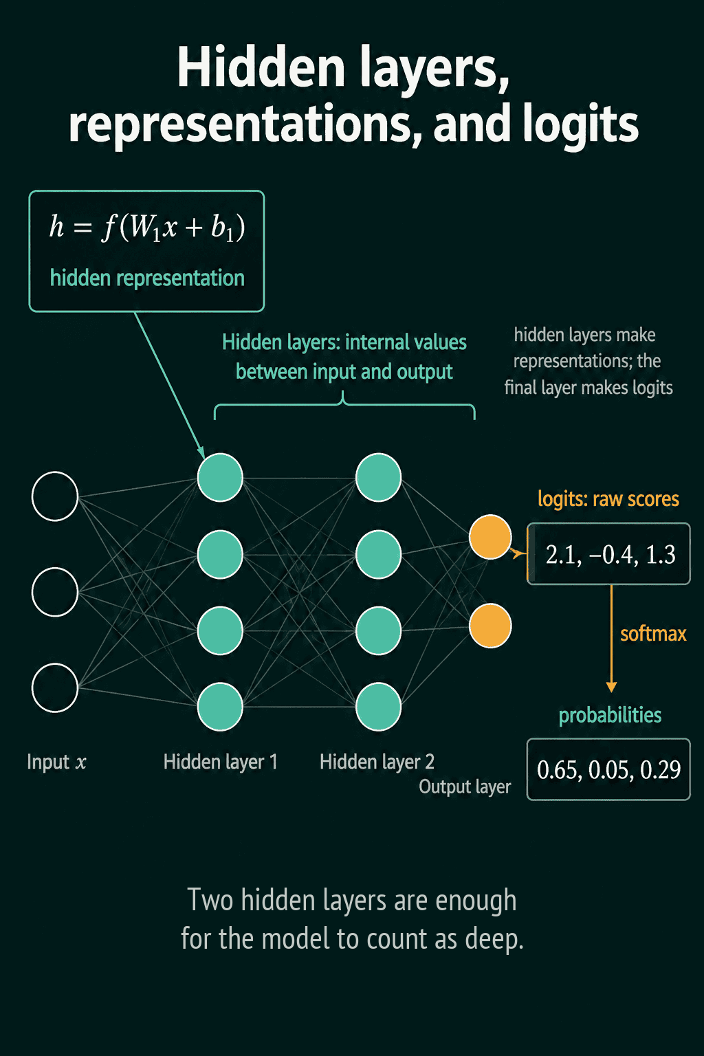
Hidden layer: any layer that is neither the input nor the output. It is called hidden because someone using the model sees the input and the final prediction, while the values in between stay inside the model.

Hidden representation: the list of numbers a hidden layer outputs, $\mathbf{h}$ in the equations above. It is the input rewritten in a form the next layer can use, and each extra layer gets another chance to rewrite it.

Logits: in a classification network, the raw scores the output layer produces, one per class. They can be any real number, such as 2.1, -0.4, and 1.3. Softmax turns a list of logits into probabilities that are between 0 and 1 and add up to 1, here 0.65, 0.05, and 0.29 (for a single yes-or-no output, sigmoid plays the same role). Hidden layers produce hidden representations, and the final layer produces logits.

A model with one layer of weights and no hidden layer is called shallow. A network with a single hidden layer is still called shallow, and two or more hidden layers make it deep.

An MLP with an input layer, two hidden layers, and an output layer, where the first hidden layer's output is labeled h equals f of W1 x plus b1, the output layer's logits 2.1, -0.4, 1.3 pass through softmax to give probabilities 0.65, 0.05, 0.29.

Why depth helps

A result called the universal approximation theorem says that one hidden layer, given enough neurons and a suitable activation, can approximate any continuous function over a bounded range of inputs as closely as you want. So why do real networks use many layers instead of one very wide one?

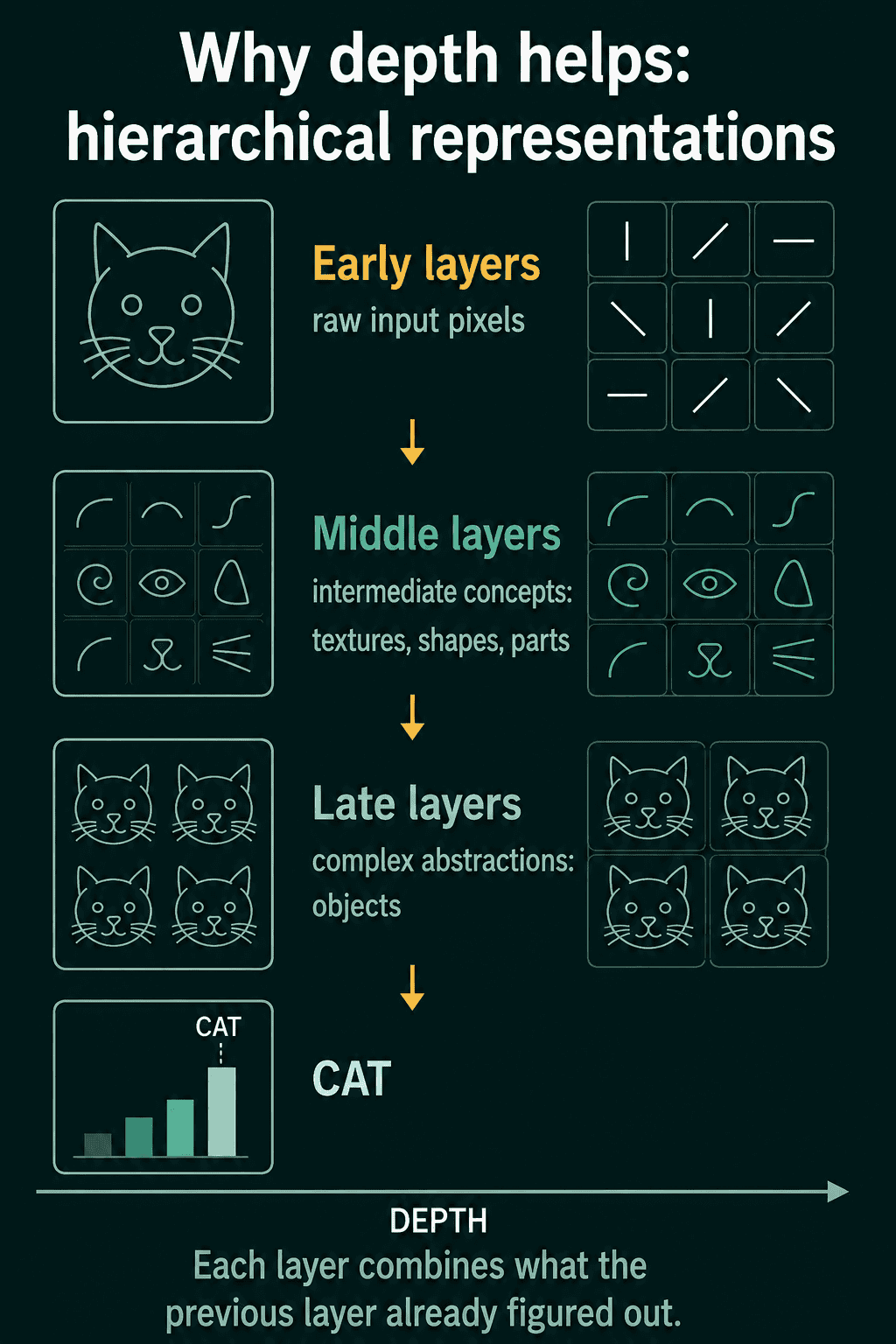
Depth lets a network build hierarchical representations, where each layer combines what the layer before it found. In an image model:

Early layers respond to simple patterns in the raw pixels, such as edges at different angles.
Middle layers combine edges into textures, shapes, and parts, such as an eye or an ear.
Late layers combine parts into whole objects, such as a cat's face.

Text and audio models show the same pattern with their own building blocks: character groups, then words, then sentences.

A wide shallow network has to learn the whole mapping from pixels to "cat" in one step. A deep network splits it up, so each layer only has to learn how to combine the previous layer's output. In practice, adding depth tends to buy more than adding width for the same number of parameters, which is why most architectures grow deep before they grow wide.

Why depth helps: early layers pick up edges from raw pixels, middle layers combine them into shapes and parts like eyes and ears, late layers combine those into whole cat faces, and the output scores the class CAT.

How to count the parameters of an MLP

Every weight and every bias is one parameter. A layer with $n_{\text{in}}$ inputs and $n_{\text{out}}$ outputs has an $n_{\text{out}} \times n_{\text{in}}$ weight matrix and one bias per output neuron:

$$\text{params} = n_{\text{in}} \times n_{\text{out}} + n_{\text{out}}$$

Count them for an MLP with 4 inputs, two hidden layers of 8 neurons, and 1 output:

Layer 1 (4 to 8): $8 \times 4 = 32$ weights plus 8 biases, 40 parameters.
Layer 2 (8 to 8): $8 \times 8 = 64$ weights plus 8 biases, 72 parameters.
Output layer (8 to 1): $1 \times 8 = 8$ weights plus 1 bias, 9 parameters.

$$\text{total} = 40 + 72 + 9 = 121$$

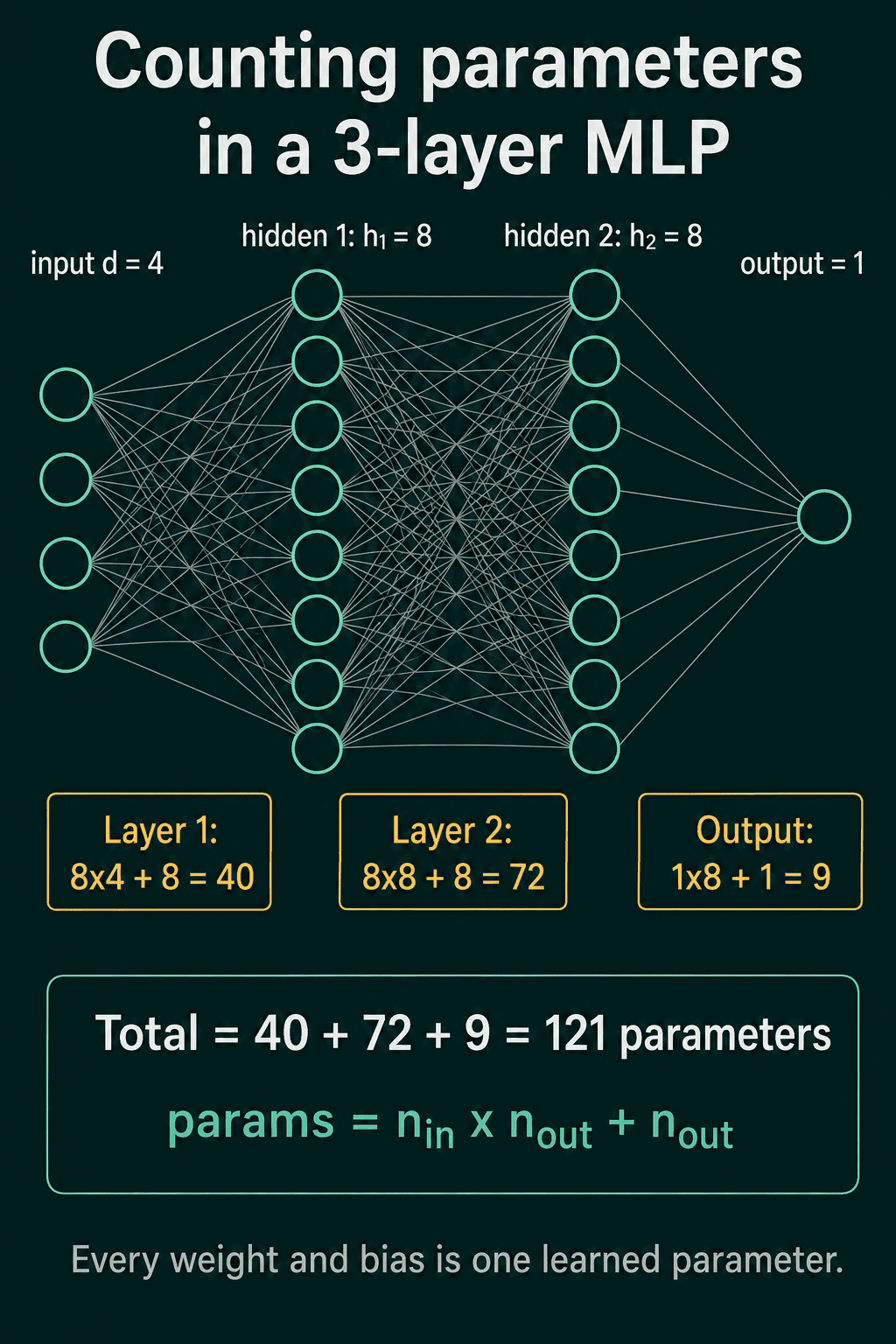
A 3-layer MLP with 4 inputs, two hidden layers of 8 neurons, and 1 output, with the counts 8x4 + 8 = 40, 8x8 + 8 = 72, and 1x8 + 1 = 9 adding up to 121 parameters.

The weight term grows with the product of the two layer widths, so doubling both widths multiplies the weights by four. One layer from 1,000 neurons to 1,000 neurons has $1000 \times 1000 + 1000 = 1{,}001{,}000$ parameters by itself, and large networks reach billions this way.

An MLP in PyTorch

This builds the 4-8-8-1 network from the count above, runs a batch through it, and checks the count:

1import torch
2import torch.nn as nn
3 
4class MLP(nn.Module):
5    def __init__(self, in_features, hidden_dim, out_features):
6        super().__init__()
7        self.layer1 = nn.Linear(in_features, hidden_dim)
8        self.layer2 = nn.Linear(hidden_dim, hidden_dim)
9        self.output = nn.Linear(hidden_dim, out_features)
10 
11    def forward(self, x):
12        h1 = torch.relu(self.layer1(x))   # first hidden representation
13        h2 = torch.relu(self.layer2(h1))  # second hidden representation
14        return self.output(h2)            # raw output, no activation
15 
16model = MLP(in_features=4, hidden_dim=8, out_features=1)
17x = torch.randn(32, 4)                    # 32 examples, 4 features each
18print(model(x).shape)
19 
20for name, p in model.named_parameters():
21    print(name, tuple(p.shape), p.numel())
22 
23print("total", sum(p.numel() for p in model.parameters()))
24 
25# torch.Size([32, 1])
26# layer1.weight (8, 4) 32
27# layer1.bias (8,) 8
28# layer2.weight (8, 8) 64
29# layer2.bias (8,) 8
30# output.weight (1, 8) 8
31# output.bias (1,) 1
32# total 121

nn.Linear(n_in, n_out) holds one weight matrix of shape (n_out, n_in) and one bias vector, and includes the bias by default. p.numel() returns how many numbers a tensor holds, so summing it over model.parameters() gives the same 121 as the hand count. If the forward pass fails with a shape error, check first that the input's last dimension equals in_features.

Common mistakes

Leaving out the activation. h = self.layer1(x) followed by self.layer2(h) is two linear layers that collapse into one, and the model can only draw a straight boundary no matter how many layers it has.
Putting an activation on the output layer. The output layer usually returns raw values. For classification, nn.CrossEntropyLoss expects logits and applies softmax internally, so a ReLU or softmax on the output changes what the loss sees.
Mismatched input size. nn.Linear does not infer its input size. A model built with in_features=4 and given a (32, 8) batch raises mat1 and mat2 shapes cannot be multiplied.
Counting parameters the wrong way. len(list(model.parameters())) counts tensors (6 for the network above), and p.shape[0] counts only the first dimension of each tensor. p.numel() counts every number.

The perceptron is a single neuron with a hard 0-or-1 output, and its straight-line limit is the reason MLPs exist. Logistic regression is a one-layer network with a sigmoid on its output, which makes it a shallow model. Backpropagation is how the gradients for all 121 parameters, or 121 billion, get computed, covered in what is backpropagation. Parameters versus hyperparameters: the weights and biases are learned, while choices like hidden_dim and the number of layers are set by you before training. The universal approximation theorem says a single wide hidden layer can approximate a continuous function as closely as needed, without saying how to find the weights, and parameters vs hyperparameters separates the 121 learned numbers from the choices, like the layer widths, made by hand.

QuiddityML teaches the multilayer perceptron and parameter counting in Unit 2 of the ML Foundation track, with exercises that include ordering the lines of an MLP class, spotting the missing activation in its forward pass, and working out the parameter count of the 4-8-8-1 network layer by layer (quiddityml.com).