By Sagi Shaier · 9 October 2026 · 6 min read

Vector norms and distances: L1, L2, Euclidean vs Manhattan

How to compute the L1, L2 and L-infinity norms by hand, when Euclidean and Manhattan distance give different answers, why L1 and L2 penalties shrink weights differently, and the PyTorch calls for each.

A norm is a single non-negative number that measures the size of a vector, and the distance between two points is the norm of the vector between them. Nearest-neighbor classifiers and k-means clustering rank points by distance, regularization adds a norm of the weights to the loss, and normalizing an embedding divides it by its norm, so the choice of norm decides what "big" and "close" mean in each of them.

What a norm has to satisfy

A vector here is an ordered list of numbers, such as $\mathbf{v} = (3, 4)$, and its norm is written $\|\mathbf{v}\|$. There is more than one formula for it, and every one of them has to satisfy three rules:

$\|\mathbf{v}\| \geq 0$, and it equals 0 only for the zero vector.
$\|c\mathbf{v}\| = |c| \, \|\mathbf{v}\|$ for any number $c$: doubling a vector doubles its size, and flipping its sign changes nothing.
$\|\mathbf{u} + \mathbf{v}\| \leq \|\mathbf{u}\| + \|\mathbf{v}\|$, the triangle inequality. For distances built from a norm, this says going through a detour point is never shorter than going direct.

The L2 norm

The L2 norm, also called the Euclidean norm, is the straight-line size of a vector, the one a ruler would give. Square every entry $v_i$, add them up, and take the square root:

$$\|\mathbf{v}\|_2 = \sqrt{\sum_i v_i^2}$$

For $(3, 4)$ that is $\sqrt{9 + 16} = 5$. L2 is the default, so a plain $\|\mathbf{v}\|$ with no subscript usually means L2.

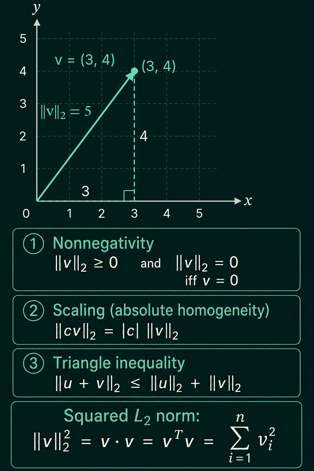
The vector v = (3, 4) drawn from the origin with L2 norm 5, above the three norm rules (nonnegativity, scaling, triangle inequality) and the identity that the squared L2 norm equals v dot v

The squared L2 norm is the dot product of the vector with itself. The dot product of two vectors multiplies their matching entries and adds the results, and for a vector paired with itself that is $\sum_i v_i^2$:

$$\|\mathbf{v}\|_2^2 = \mathbf{v} \cdot \mathbf{v}$$

Unit vectors and normalizing

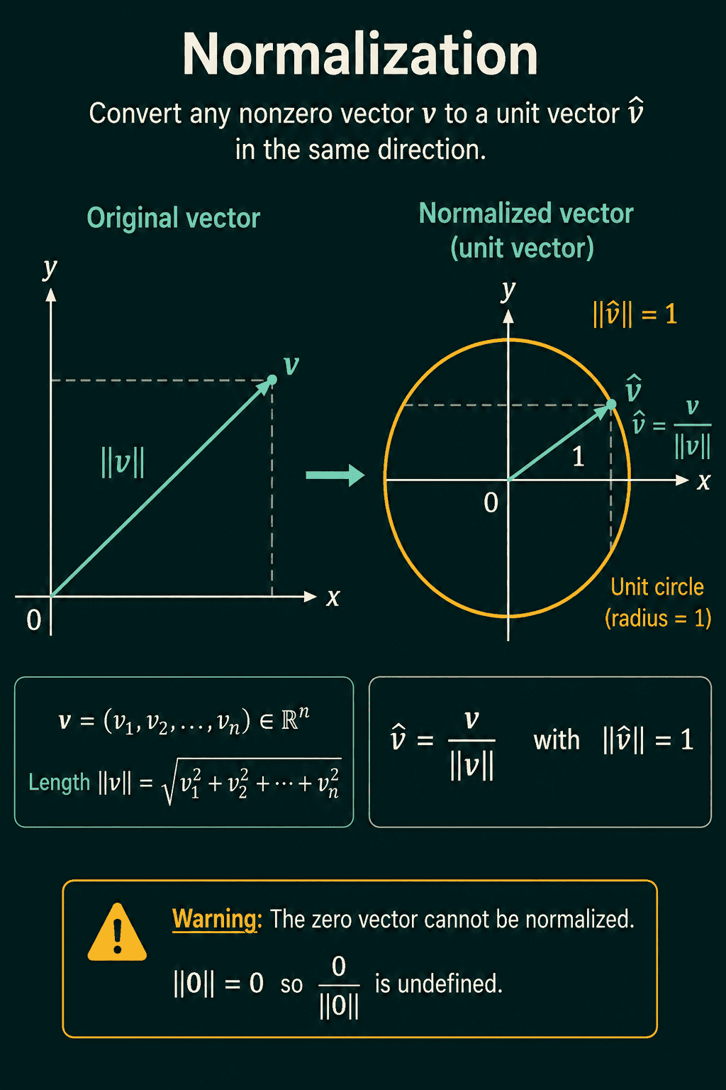
A vector with norm exactly 1 is a unit vector. Dividing any nonzero vector by its own norm gives one, pointing in the same direction:

$$\hat{\mathbf{v}} = \frac{\mathbf{v}}{\|\mathbf{v}\|}$$

That step is called normalizing, and in PyTorch it is v / v.norm(). $(3, 4)$ becomes $(0.6, 0.8)$. After normalizing, the length carries no information, so anything measured with $\hat{\mathbf{v}}$ is about direction alone. The zero vector cannot be normalized, since its norm is 0 and dividing by 0 has no answer.

Left: an original vector v with length marked. Right: the normalized vector v hat = v divided by its length, ending on the unit circle with length 1. Below: the length formula and a warning that the zero vector cannot be normalized

The L1 and L-infinity norms

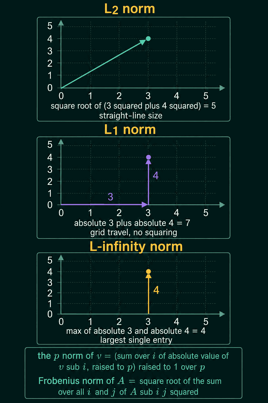
The L1 norm adds up the absolute values of the entries, with no squaring:

$$\|\mathbf{v}\|_1 = \sum_i |v_i|$$

For $(3, 4)$ that is $3 + 4 = 7$. L1 counts every unit of movement along every axis at full weight. L2 squares each entry first, which lets large entries dominate and shrinks small ones, so L2 penalizes one big entry much more than several small ones.

The L-infinity norm keeps only the largest absolute entry:

$$\|\mathbf{v}\|_\infty = \max_i |v_i|$$

For $(3, 4)$ that is 4.

The vector (3, 4) measured three ways: L2 as the straight line of length 5, L1 as 3 along plus 4 up for 7, and L-infinity as the largest single entry, 4, with the p-norm and Frobenius formulas written underneath

For any vector the three come out in the same order:

$$\|\mathbf{v}\|_\infty \leq \|\mathbf{v}\|_2 \leq \|\mathbf{v}\|_1$$

L-infinity keeps one term out of a sum of non-negative numbers, so it is never the largest. For $(3, 4)$ the order reads $4 \leq 5 \leq 7$.

The p-norm family and the Frobenius norm

L1, L2 and L-infinity are three members of one family, the $\ell_p$ norm, set by a number $p$:

$$\|\mathbf{v}\|_p = \Big(\sum_i |v_i|^p\Big)^{1/p}$$

$p = 1$ gives L1 and $p = 2$ gives L2. As $p$ grows toward infinity, the largest entry dominates the sum more and more, and the expression approaches $\max_i |v_i|$, the L-infinity norm. Other values of $p$ rarely come up in machine learning.

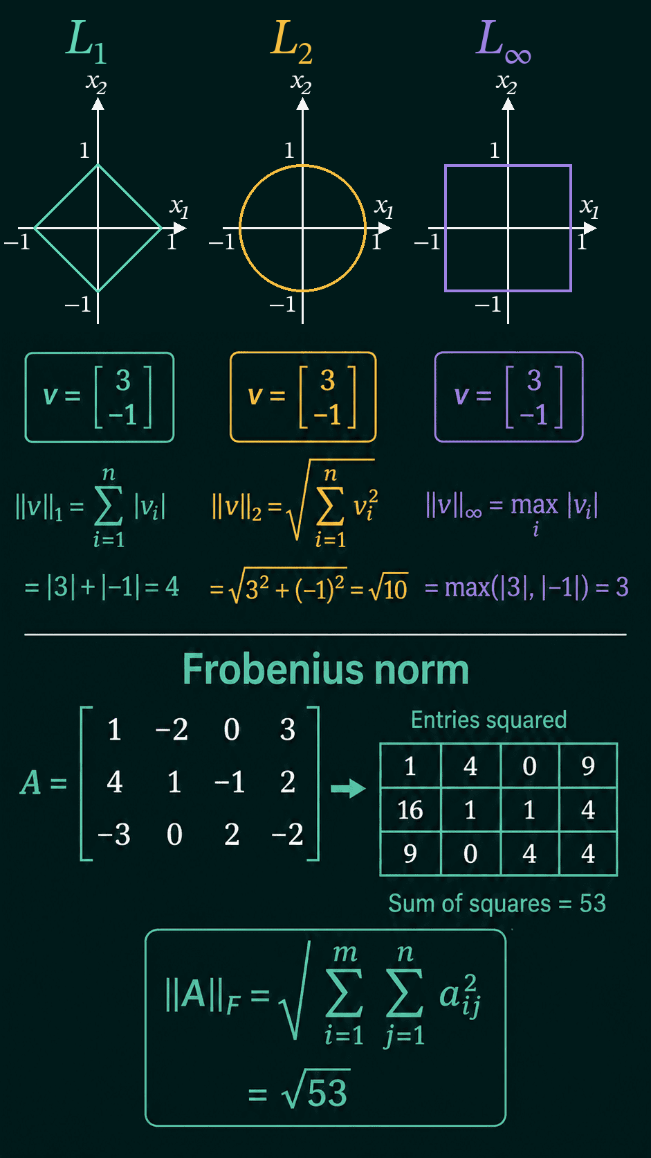
The Frobenius norm is L2 applied to a matrix: square every entry of the matrix $A$, add them all, and take the square root. $A_{ij}$ is the entry in row $i$ and column $j$:

$$\|A\|_F = \sqrt{\sum_{i,j} A_{ij}^2}$$

The set of all 2D points with norm exactly 1 takes a different shape under each norm: a diamond for L1, a circle for L2, and a square for L-infinity. For $\mathbf{v} = (3, -1)$ the three norms come out as $4$, $\sqrt{10}$ and $3$.

Top: the points with norm 1 under L1, L2 and L-infinity, drawn as a diamond, a circle and a square, with the three norms of v = (3, -1) computed as 4, the square root of 10, and 3. Bottom: a 3 by 4 matrix whose squared entries sum to 53, so its Frobenius norm is the square root of 53

From norms to distances

The distance between two points $\mathbf{p}$ and $\mathbf{q}$ is the norm of the vector between them, $\mathbf{p} - \mathbf{q}$. With the L2 norm this is the Euclidean distance, the straight-line distance:

$$d(\mathbf{p}, \mathbf{q}) = \|\mathbf{p} - \mathbf{q}\|_2$$

$$= \sqrt{\sum_i (p_i - q_i)^2}$$

Swap in the L1 norm and the result is the Manhattan distance: the sum of the differences along each axis, the distance traveled when you can only move along the grid lines. For $\mathbf{p} = (1, 1)$ and $\mathbf{q} = (5, 4)$, the differences are 4 and 3, so the Euclidean distance is $\sqrt{16 + 9} = 5$ and the Manhattan distance is $4 + 3 = 7$.

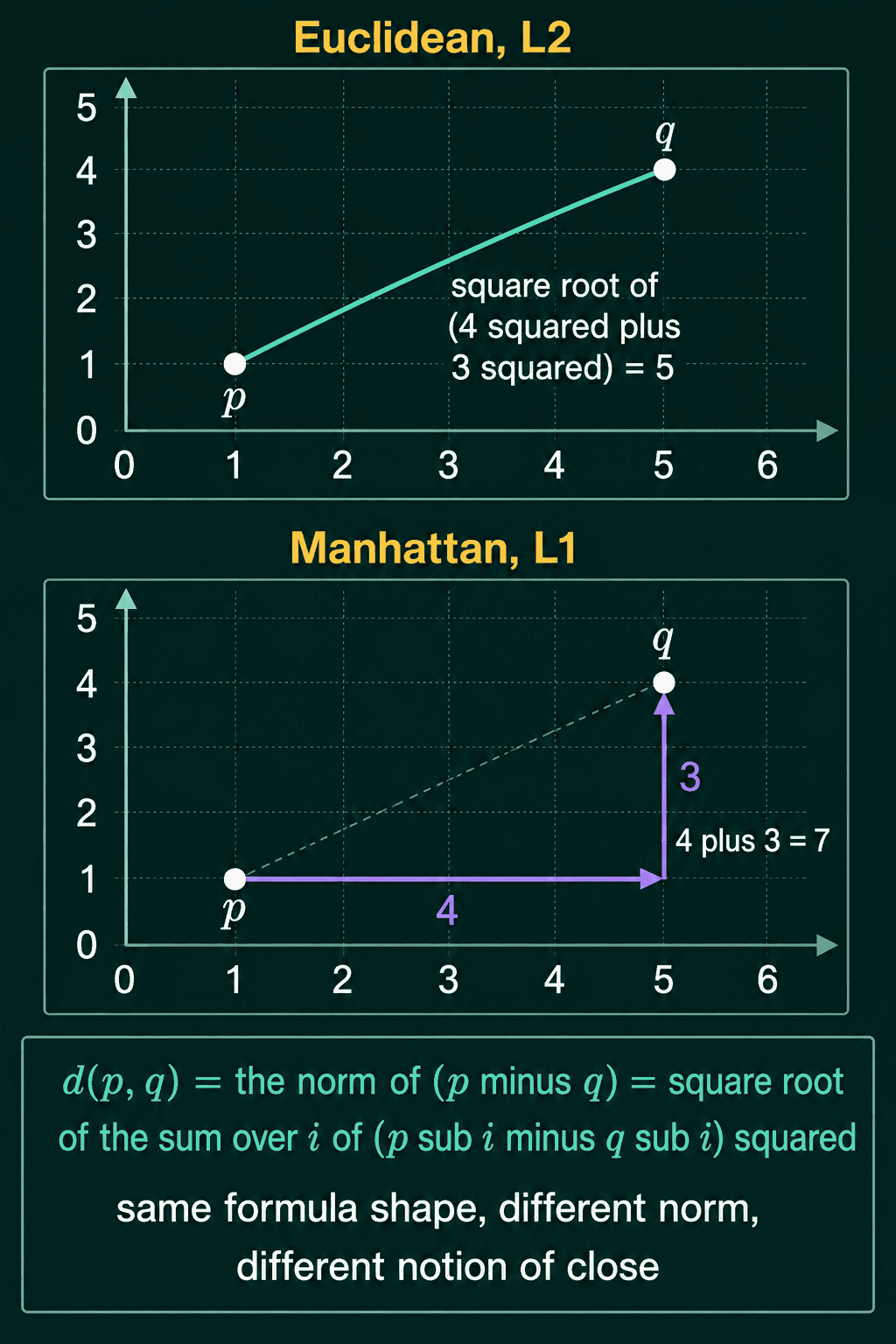
Points p = (1, 1) and q = (5, 4): the Euclidean (L2) distance is the straight line of length 5, and the Manhattan (L1) distance is 4 along plus 3 up for 7

A vector's length is the Euclidean distance from the origin to the point it describes. k-nearest neighbors classifies a new point by finding the training points with the smallest distance to it. k-means clustering groups points by minimizing their distance to a cluster center. Comparing two embeddings often uses this distance too.

Norms as regularizers

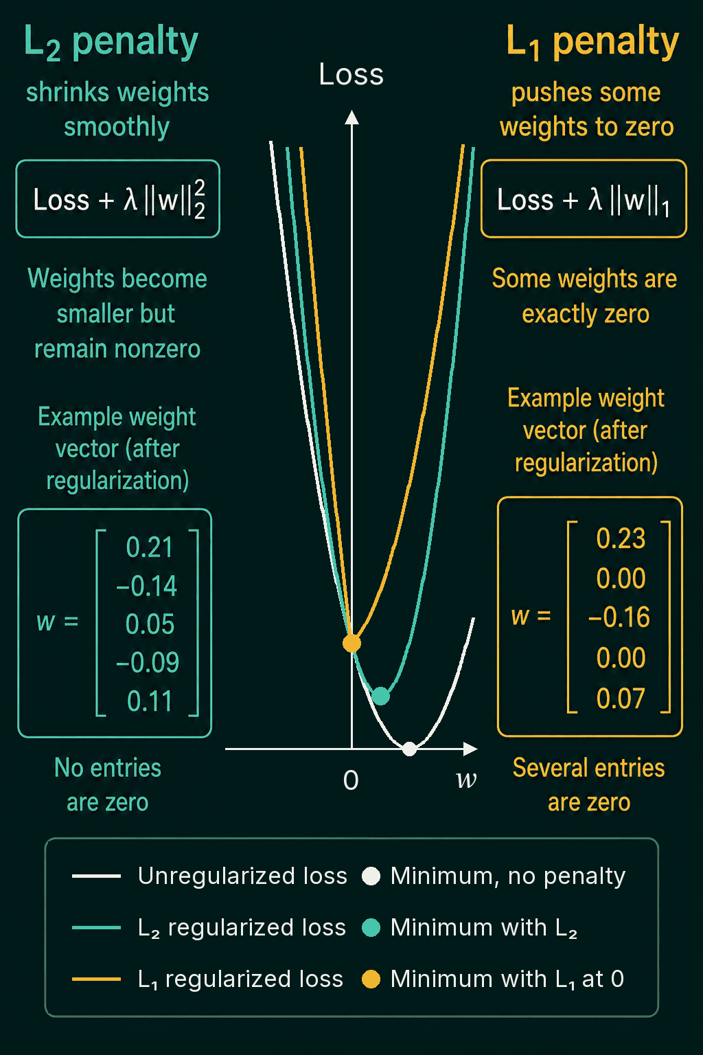
Regularization adds a penalty on the size of the weights $\mathbf{w}$ to the training loss, so the optimizer is pushed toward smaller weights. The size is measured with a norm, and the two common choices behave differently:

L2 regularization adds $\|\mathbf{w}\|_2^2$. Because squaring shrinks small values, the penalty eases off as a weight gets close to zero, so weights get smaller but usually stay nonzero. With plain SGD it is equivalent to weight decay, though the two behave differently with an adaptive optimizer like Adam.
L1 regularization adds $\|\mathbf{w}\|_1$. It pushes on small weights as hard as on large ones, so it tends to drive some weights to exactly zero.

The number $\lambda$ (lambda) in front of the penalty sets how strongly it counts against the loss. For a model with a single weight $w$ whose loss is lowest at a positive value, adding the L2 penalty moves the lowest point closer to 0, and adding a large enough L1 penalty moves it to exactly 0.

A loss curve over one weight w with its minimum at a positive w, the same loss plus an L2 penalty with its minimum moved closer to 0, and the same loss plus an L1 penalty with its minimum at exactly 0, next to example weight vectors: no zero entries under L2, several exact zeros under L1

Norms and distances in PyTorch

1import torch
2 
3v = torch.tensor([3.0, 4.0])
4print(torch.linalg.vector_norm(v, ord=1))             # L1
5print(torch.linalg.vector_norm(v))                    # L2, the default
6print(torch.linalg.vector_norm(v, ord=float("inf")))  # L-infinity
7print(v @ v, v.norm() ** 2)                           # squared L2 = v . v
8 
9v_hat = v / v.norm()
10print(v_hat, v_hat.norm())
11 
12A = torch.tensor([[1.0, -2.0, 0.0, 3.0],
13                  [4.0, 1.0, -1.0, 2.0],
14                  [-3.0, 0.0, 2.0, -2.0]])
15print(torch.linalg.matrix_norm(A), 53 ** 0.5)         # Frobenius, the default

1tensor(7.)
2tensor(5.)
3tensor(4.)
4tensor(25.) tensor(25.)
5tensor([0.6000, 0.8000]) tensor(1.)
6tensor(7.2801) 7.280109889280518

Distances are the norm of a difference, and torch.cdist computes the distance from every point in one set to every point in another, which is the core step of nearest neighbors:

1import torch
2 
3p = torch.tensor([1.0, 1.0])
4q = torch.tensor([5.0, 4.0])
5print(torch.linalg.vector_norm(p - q))         # Euclidean, L2
6print(torch.linalg.vector_norm(p - q, ord=1))  # Manhattan, L1
7 
8# nearest neighbor: distance from one new point to every training point
9train = torch.tensor([[0.0, 0.0], [5.0, 4.0], [2.0, 1.0], [6.0, 6.0]])
10new = torch.tensor([[1.0, 1.0]])
11d = torch.cdist(new, train)                    # p=2 by default
12print(d)
13print(d.argmin().item())

1tensor(5.)
2tensor(7.)
3tensor([[1.4142, 5.0000, 1.0000, 7.0711]])
42

The closest training point is index 2, $(2, 1)$, at distance 1. torch.cdist(new, train, p=1) switches it to Manhattan distance.

Adding a regularizer is one extra term in the loss:

1import torch
2 
3torch.manual_seed(0)
4model = torch.nn.Linear(10, 1)
5x, y = torch.randn(32, 10), torch.randn(32, 1)
6lam = 1e-3
7 
8loss = torch.nn.functional.mse_loss(model(x), y)
9l2 = model.weight.pow(2).sum()      # squared L2 norm of the weights
10l1 = model.weight.abs().sum()       # L1 norm of the weights
11total = loss + lam * l2             # swap in l1 for L1 regularization
12total.backward()

If the model stops learning after adding the penalty, lower lam first, since a large $\lambda$ lets the penalty outweigh the loss.

Common mistakes

Assuming "norm" means L2 everywhere. torch.linalg.vector_norm defaults to L2, but a paper or library may mean L1 or L-infinity, so check the subscript or the ord argument.
Mixing up $\|\mathbf{w}\|_2$ and $\|\mathbf{w}\|_2^2$. L2 regularization uses the squared norm, which has no square root.
Normalizing a zero vector. v / v.norm() on a zero vector gives nan in every entry.
Comparing distances across different norms. A Manhattan distance of 7 and a Euclidean distance of 5 can describe the same two points.

The dot product gives the squared L2 norm of a vector paired with itself, and is covered in the dot product explained. Cosine similarity divides the dot product by two L2 norms to compare direction alone, covered in cosine similarity explained.

QuiddityML teaches norms and distances as their own concepts in the linear algebra part of the Math track, and the exercises include turning the L1, L2 and distance formulas into code, spotting the bug in an l1_norm and l2_norm pair, and writing a distance function from scratch.