By Sagi Shaier · 9 October 2026 · 7 min read

Orthogonality explained: orthogonal matrices, orthonormal bases, and projections

How to tell when two vectors or a whole matrix are orthogonal, why the inverse of an orthogonal matrix is its transpose, how to project one vector onto another, and how Gram-Schmidt builds an orthonormal basis, with PyTorch code for each.

Two vectors are orthogonal when they sit at a right angle to each other, which happens exactly when their dot product is zero. The idea scales up to matrices whose columns are all at right angles, to bases built from right-angled unit vectors, and to projections that split a vector into a part along a direction and a part at a right angle to it. Orthogonal weight initialization, least squares regression, PCA and the QR factorization are all built on these pieces.

Orthogonal vectors

The dot product of two vectors $\mathbf{u}$ and $\mathbf{v}$ multiplies their matching entries and adds the results: $\mathbf{u} \cdot \mathbf{v} = \sum_i u_i v_i$. It also equals $\|\mathbf{u}\| \|\mathbf{v}\| \cos(\theta)$, where $\|\mathbf{u}\|$ is the length of $\mathbf{u}$ and $\theta$ is the angle between the two vectors. At a right angle $\cos(\theta) = 0$, so:

$$\mathbf{u} \perp \mathbf{v} \iff \mathbf{u} \cdot \mathbf{v} = 0$$

The symbol $\perp$ means "is orthogonal to". $(0, 1)$ and $(1, 0)$ are orthogonal, since $0 \times 1 + 1 \times 0 = 0$.

Orthogonal matrices

An orthogonal matrix is a square matrix $Q$ whose columns all have length 1 and are all orthogonal to each other. Columns with both properties are called orthonormal. Checking every pair of columns by hand is slow, and one matrix equation does it at once:

$$Q^\top Q = I$$

$Q^\top$ is the transpose of $Q$ (rows and columns swapped), and $I$ is the identity matrix, with 1s on the diagonal and 0s everywhere else. Each entry of $Q^\top Q$ is the dot product of two columns of $Q$: the diagonal entries are each column with itself, which is its squared length and has to be 1, and the off-diagonal entries are pairs of different columns, which have to be 0.

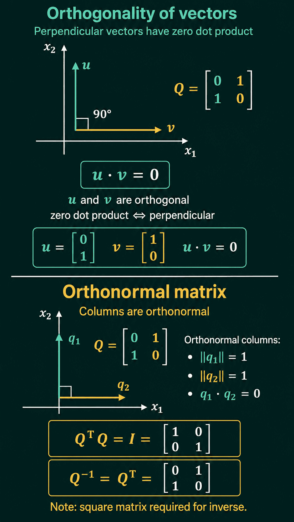
Top: u = (0, 1) and v = (1, 0) at a right angle with dot product 0. Bottom: a 2 by 2 matrix whose columns q1 and q2 each have length 1 and dot product 0, so Q transpose Q is the identity and the inverse of Q is Q transpose

$Q^\top Q = I$ says that $Q^\top$ undoes $Q$, so the inverse of an orthogonal matrix is its transpose:

$$Q^{-1} = Q^\top$$

Computing an inverse is usually expensive, and for an orthogonal matrix it costs nothing more than swapping rows and columns. This step needs $Q$ to be square. A tall matrix with more rows than columns can have orthonormal columns and satisfy $Q^\top Q = I$, but a non-square matrix has no inverse.

Rotations, reflections, and stable initialization

Orthogonal matrices are the rotations and reflections: they change the direction of a vector and leave its length alone. For every vector $\mathbf{x}$:

$$\|Q\mathbf{x}\| = \|\mathbf{x}\|$$

The matrix with rows $(0, -1)$ and $(1, 0)$ rotates every vector by 90 degrees. It sends $(3, 4)$ to $(-4, 3)$, and both have length 5.

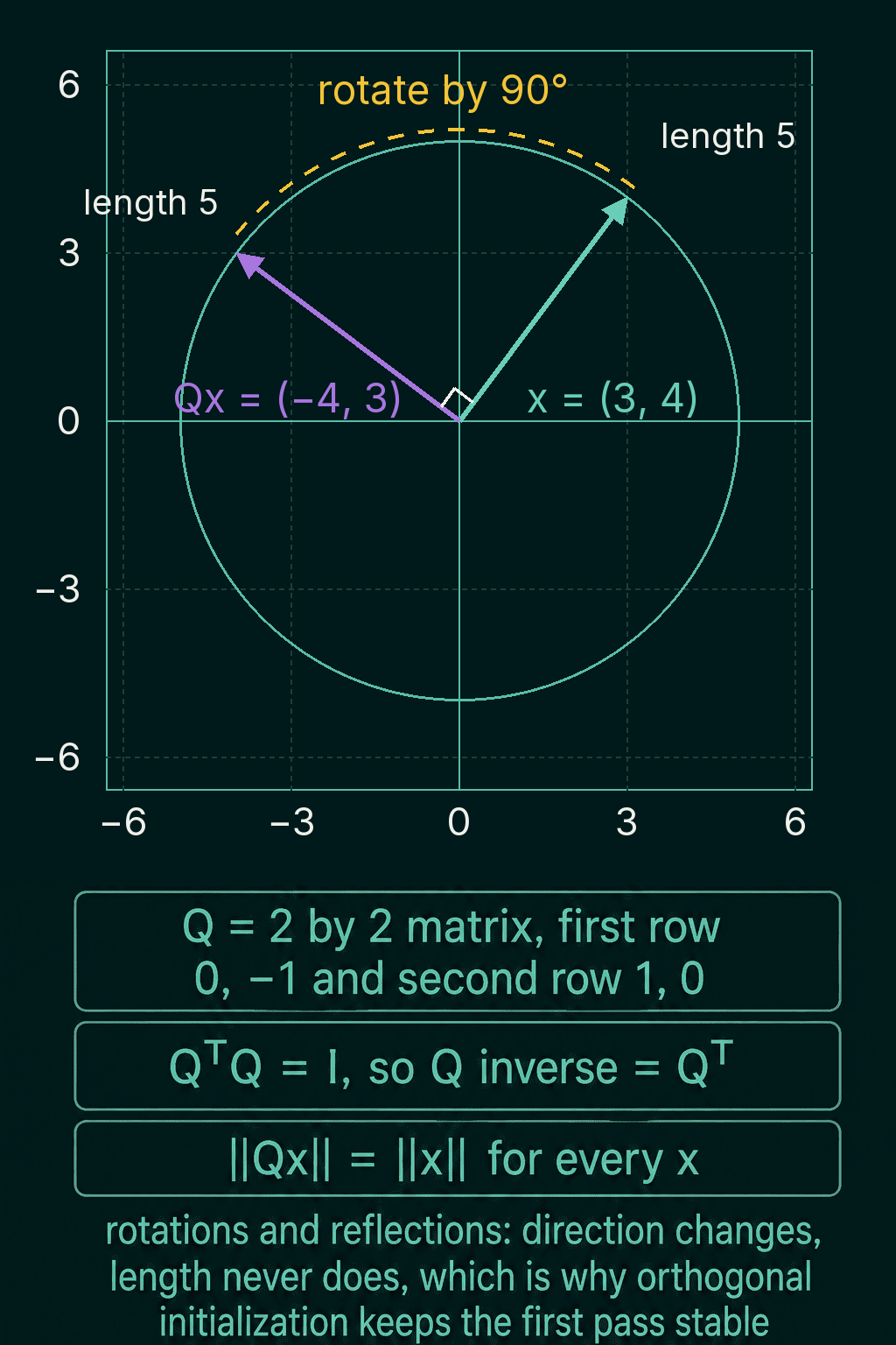
The vector x = (3, 4) and its rotation Qx = (-4, 3), both ending on the circle of radius 5, with Q the 90 degree rotation matrix with rows (0, -1) and (1, 0), Q transpose Q = I, and the length of Qx equal to the length of x

Because they keep lengths, orthogonal matrices are used to initialize the weights of a layer. A layer whose weight matrix is orthogonal neither shrinks nor inflates the scale of its input on the first forward and backward pass, which helps training start off stable.

A unitary matrix is the version for complex numbers: $U^*U = I$, where $U^*$ is the conjugate transpose (transpose, then flip the sign of every imaginary part). For a real matrix, unitary and orthogonal mean the same thing.

Projecting one vector onto another

The projection of a vector $\mathbf{v}$ onto a direction $\mathbf{u}$ is the point on the line through $\mathbf{u}$ that is closest to $\mathbf{v}$. It is written $\text{proj}_{\mathbf{u}}(\mathbf{v})$:

$$\text{proj}_{\mathbf{u}}(\mathbf{v}) = \frac{\mathbf{v} \cdot \mathbf{u}}{\mathbf{u} \cdot \mathbf{u}} \, \mathbf{u}$$

The fraction is a single number that says how far to travel along $\mathbf{u}$, and multiplying $\mathbf{u}$ by it lands on the projected point. The denominator $\mathbf{u} \cdot \mathbf{u}$ is the squared length $\|\mathbf{u}\|^2$.

For $\mathbf{v} = (1, 3)$ and $\mathbf{u} = (3, 1)$: $\mathbf{v} \cdot \mathbf{u} = 3 + 3 = 6$ and $\mathbf{u} \cdot \mathbf{u} = 9 + 1 = 10$, so the projection is $0.6 \times (3, 1) = (1.8, 0.6)$.

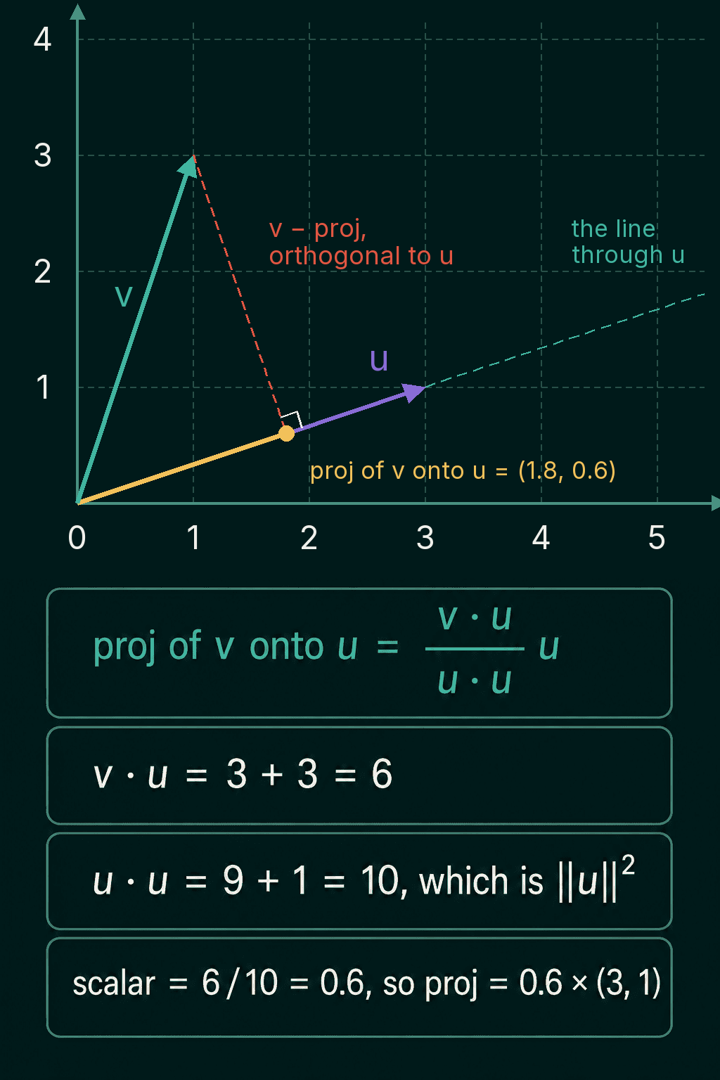
v = (1, 3) and u = (3, 1), with the projection of v onto u at (1.8, 0.6) on the line through u, and the leftover piece from the projection to v drawn at a right angle to u, above the worked calculation 6 / 10 = 0.6

The leftover piece, $\mathbf{v} - \text{proj}_{\mathbf{u}}(\mathbf{v})$, is always orthogonal to $\mathbf{u}$. Here it is $(-0.8, 2.4)$, and $(-0.8) \times 3 + 2.4 \times 1 = 0$. A projection therefore splits $\mathbf{v}$ into a part along $\mathbf{u}$ and a part at a right angle to it. Least squares regression projects the target values onto the space the feature columns can reach, and PCA projects data onto a few right-angled unit directions that capture the most variance.

Orthonormal bases

A basis is a set of vectors that can build every vector in a space through scaling and adding, with none of them redundant. A basis is orthonormal when every basis vector has length 1 and every pair is orthogonal. $(1, 0)$ and $(0, 1)$ form an orthonormal basis for 2D space, and so does any pair you get by rotating both of them together.

Finding the coordinates of a vector in a general basis means solving a system of equations. In an orthonormal basis each coordinate is one dot product: the coefficient for basis vector $\mathbf{e}_i$ is $\mathbf{v} \cdot \mathbf{e}_i$.

With $\mathbf{e}_1 = (0.71, 0.71)$ and $\mathbf{e}_2 = (-0.71, 0.71)$, the vector $(2, 1)$ has coordinates $2 \times 0.71 + 1 \times 0.71 = 2.12$ and $2 \times (-0.71) + 1 \times 0.71 = -0.71$, so $(2, 1) = 2.12\,\mathbf{e}_1 - 0.71\,\mathbf{e}_2$.

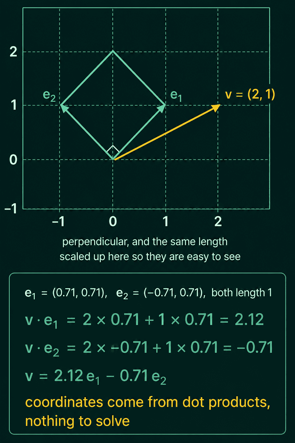
The rotated orthonormal basis e1 = (0.71, 0.71) and e2 = (-0.71, 0.71), drawn scaled up, and the vector v = (2, 1), with its coordinates computed as the dot products 2.12 and -0.71

The columns of every orthogonal matrix form an orthonormal basis.

Building an orthonormal basis with Gram-Schmidt

Gram-Schmidt turns an ordinary basis $\mathbf{v}_1, \dots, \mathbf{v}_n$ into an orthonormal one. Take the vectors in order. For each $\mathbf{v}_k$, subtract its projection onto every unit vector $\mathbf{e}_j$ already built, then divide what is left by its length:

$$\mathbf{w}_k = \mathbf{v}_k - \sum_{j<k} (\mathbf{v}_k \cdot \mathbf{e}_j)\,\mathbf{e}_j$$

$$\mathbf{e}_k = \frac{\mathbf{w}_k}{\|\mathbf{w}_k\|}$$

Each $\mathbf{e}_j$ has length 1, so its projection is $(\mathbf{v}_k \cdot \mathbf{e}_j)\,\mathbf{e}_j$ with no denominator. Subtracting every earlier projection leaves $\mathbf{w}_k$ orthogonal to all of the earlier directions, and dividing by its length makes it a unit vector.

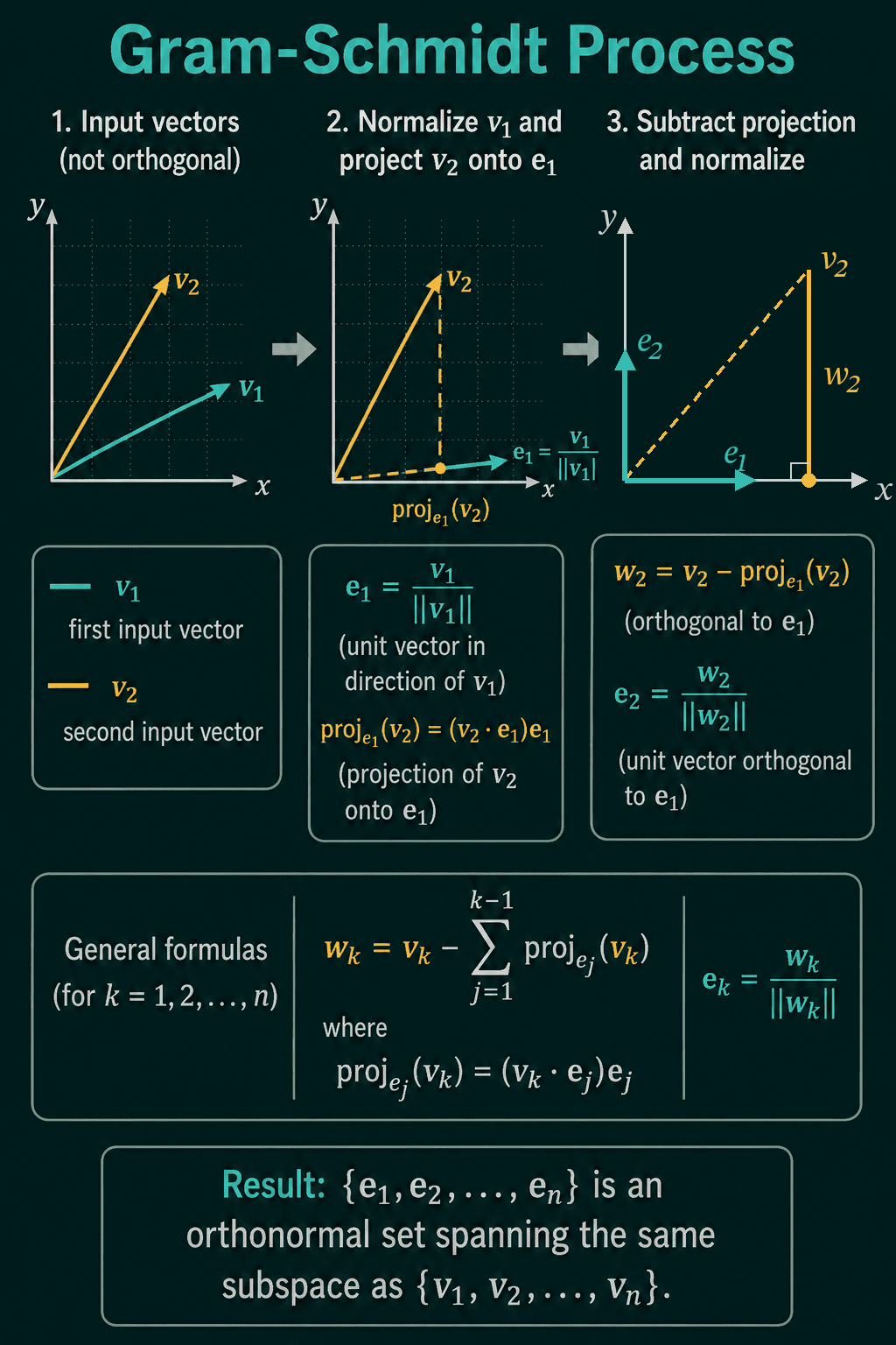
Gram-Schmidt in three steps: two input vectors v1 and v2 that are not orthogonal, then v1 normalized to e1 and v2 projected onto e1, then the projection subtracted to give w2 at a right angle to e1 and w2 normalized to e2, with the general formulas below

If $\mathbf{w}_k$ comes out as the zero vector, $\mathbf{v}_k$ was a combination of the earlier vectors and adds no new direction. The QR factorization of a matrix runs the same procedure.

Orthogonality in PyTorch

1import torch
2 
3Q = torch.tensor([[0.0, -1.0],
4                  [1.0,  0.0]])        # rotate by 90 degrees
5print(Q.T @ Q)                         # identity, so Q is orthogonal
6print(torch.linalg.inv(Q))             # the inverse ...
7print(Q.T)                             # ... is the transpose
8 
9x = torch.tensor([3.0, 4.0])
10print(Q @ x, x.norm(), (Q @ x).norm()) # direction changes, length stays 5
11 
12# orthogonal initialization of a layer's weights
13layer = torch.nn.Linear(4, 4)
14torch.nn.init.orthogonal_(layer.weight)
15W = layer.weight.detach()
16print(torch.allclose(W.T @ W, torch.eye(4), atol=1e-6))

1tensor([[1., 0.],
2        [0., 1.]])
3tensor([[ 0.,  1.],
4        [-1.,  0.]])
5tensor([[ 0.,  1.],
6        [-1.,  0.]])
7tensor([-4.,  3.]) tensor(5.) tensor(5.)
8True

Projection and coordinates in an orthonormal basis:

1import torch
2 
3def project(v, u):
4    return (v @ u) / (u @ u) * u
5 
6v = torch.tensor([1.0, 3.0])
7u = torch.tensor([3.0, 1.0])
8p = project(v, u)
9r = v - p
10print(p, r, r @ u)                     # residual is orthogonal to u
11 
12# coordinates in an orthonormal basis are dot products
13e1 = torch.tensor([1.0, 1.0]) / 2 ** 0.5
14e2 = torch.tensor([-1.0, 1.0]) / 2 ** 0.5
15w = torch.tensor([2.0, 1.0])
16c1, c2 = w @ e1, w @ e2
17print(c1, c2, c1 * e1 + c2 * e2)

1tensor([1.8000, 0.6000]) tensor([-0.8000,  2.4000]) tensor(0.)
2tensor(2.1213) tensor(-0.7071) tensor([2.0000, 1.0000])

And Gram-Schmidt on the columns $(3, 1)$ and $(2, 3)$:

1import torch
2 
3def gram_schmidt(V):
4    """Columns of V in, orthonormal columns out."""
5    E = []
6    for k in range(V.shape[1]):
7        w = V[:, k].clone()
8        for e in E:
9            w = w - (w @ e) * e        # remove the part along e
10        E.append(w / w.norm())
11    return torch.stack(E, dim=1)
12 
13V = torch.tensor([[3.0, 2.0],
14                  [1.0, 3.0]])         # columns v1 = (3, 1), v2 = (2, 3)
15E = gram_schmidt(V)
16print(E)
17print((E.T @ E).round(decimals=4))

1tensor([[ 0.9487, -0.3162],
2        [ 0.3162,  0.9487]])
3tensor([[1., 0.],
4        [0., 1.]])

The loop subtracts each projection from the running remainder w rather than from the original column, which gives the same answer and loses less precision to rounding. If $E^\top E$ comes out far from the identity, check whether two input columns were nearly parallel, since their remainder is then tiny and dividing by its length amplifies rounding errors.

Common mistakes

Calling a matrix orthogonal when its columns are only at right angles. The columns also need length 1, otherwise $Q^\top Q$ has other numbers on its diagonal.
Using $Q^\top$ as the inverse of a non-square matrix. $Q^\top Q = I$ can hold for a tall matrix, and it still has no inverse.
Dropping the denominator in the projection formula. $(\mathbf{v} \cdot \mathbf{u})\,\mathbf{u}$ is the projection only when $\mathbf{u}$ has length 1.
Reading a zero dot product as "one vector is small". It means the two directions are at a right angle.

The dot product that defines orthogonality is covered in the dot product explained, and the vector lengths used throughout are in vector norms and distances. Least squares takes the projection from one direction to a whole column space, which is how linear regression finds its best fit.

QuiddityML teaches orthogonal matrices, projections and orthonormal bases as separate concepts in the linear algebra part of the Math track, with hands-on exercises on each, from turning the projection formula into code to writing Gram-Schmidt from scratch.