By Sagi Shaier · 2 November 2026 · 10 min read
How to visualize and evaluate word embeddings: clustering, intrinsic and extrinsic evaluation
How to plot word vectors in 2D without misreading them, find a word's nearest neighbors and groups of similar words in PyTorch, and test whether a set of embeddings is any good.
Word embeddings give each token a list of numbers, learned so that tokens with similar meanings get similar numbers. A token is the unit of text a model works with, often a whole word and sometimes a piece of one, and this post says "word" to keep the examples simple. Visualizing them means squeezing those numbers down to 2 or 3 per word so the words can be plotted. Evaluating them means checking whether the numbers capture meaning, either against human judgments or inside a real task. You need both whenever you train or download embeddings and want to know what you got.
Why can't you look at an embedding directly?
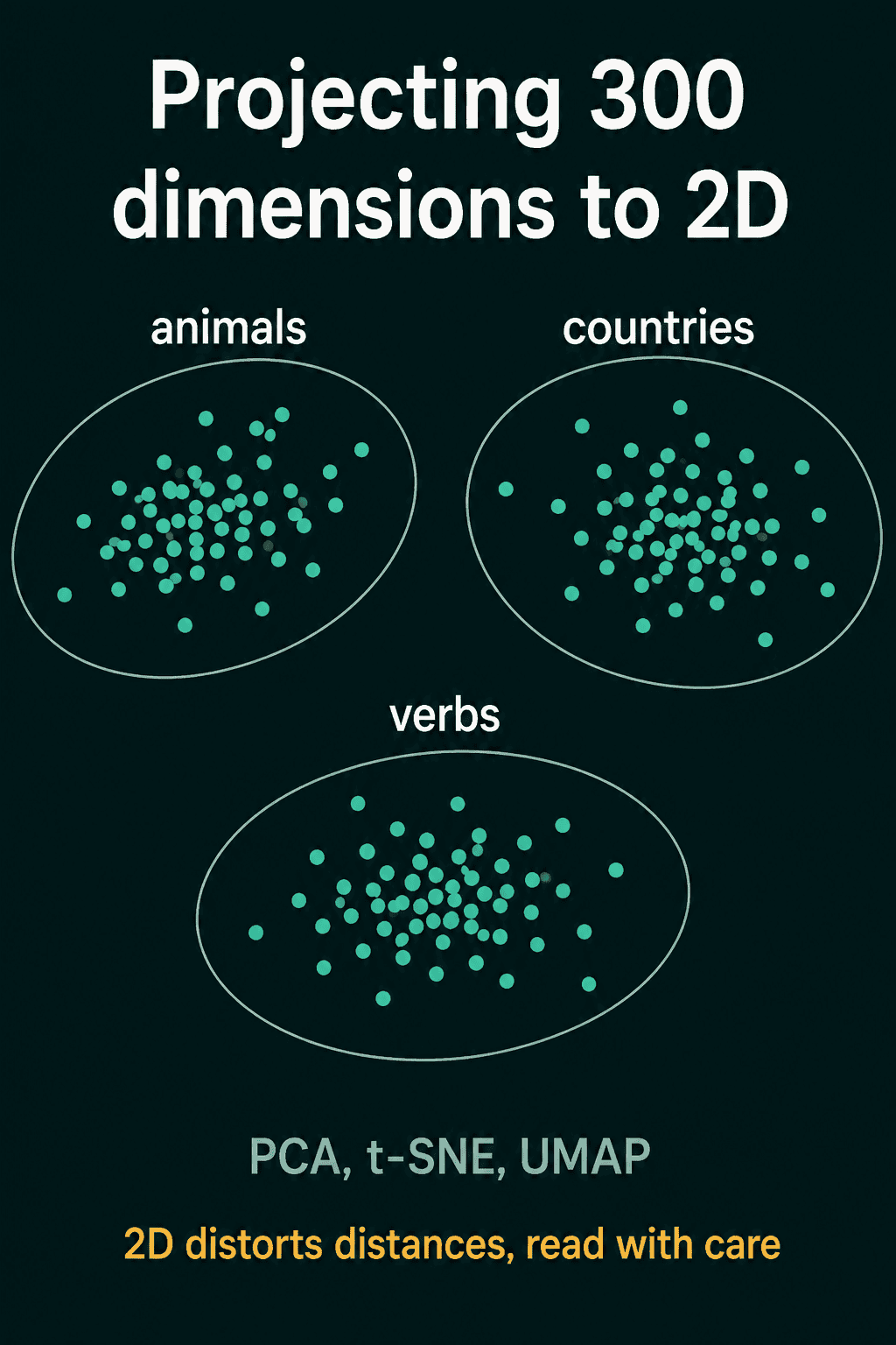
The list can be any length, and around 300 numbers per word is a common size. A person can read a point in 2 dimensions, or 3 with some effort, and a point in 300 dimensions has no picture at all. So the 300 numbers have to be reduced to 2 or 3 first, and only then plotted.
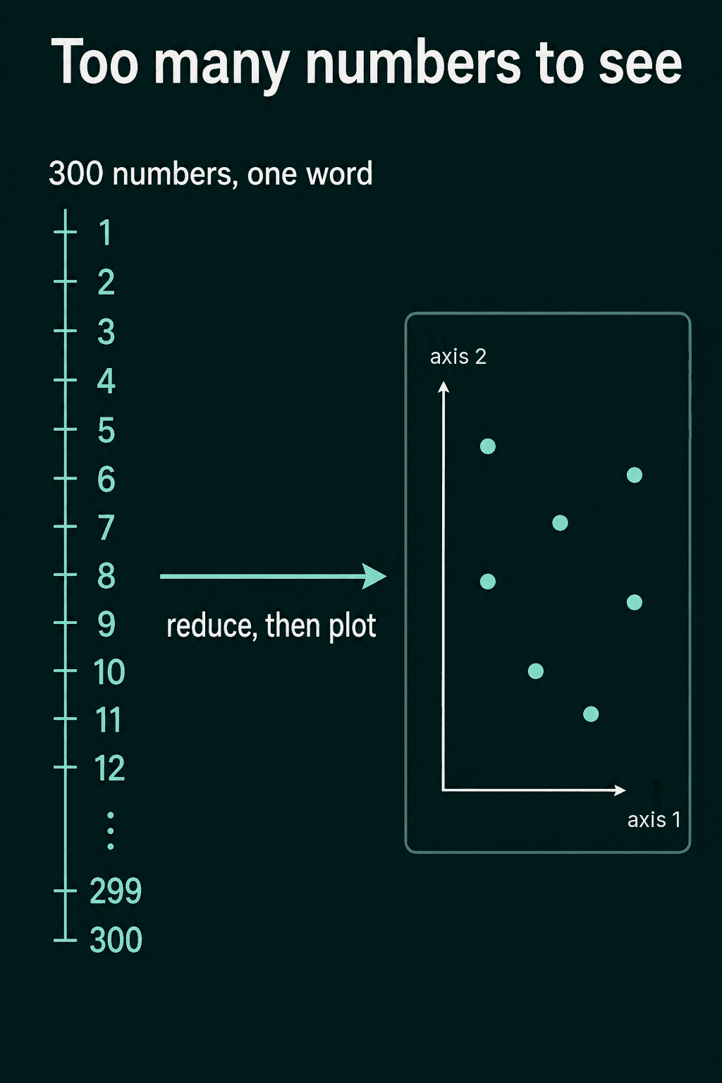
The reduction has one job: words that were close in the 300 numbers should stay close on the plot, and words that were far apart should stay far apart. Giving each word 2 random numbers would plot something, but words that were close in the real space could land anywhere and the picture would say nothing true.
Any reduction loses information, because 298 of the 300 dimensions have to go somewhere. A gap on the plot may not be a gap in the real space, and groups can look cleaner or messier than they are. Read the picture as a rough sketch, not a measurement.
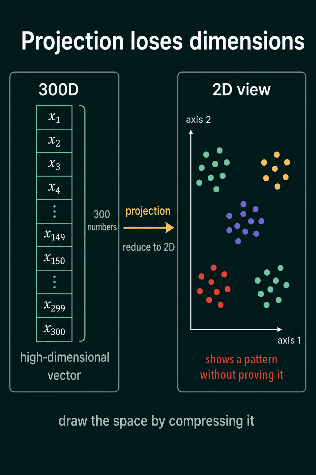
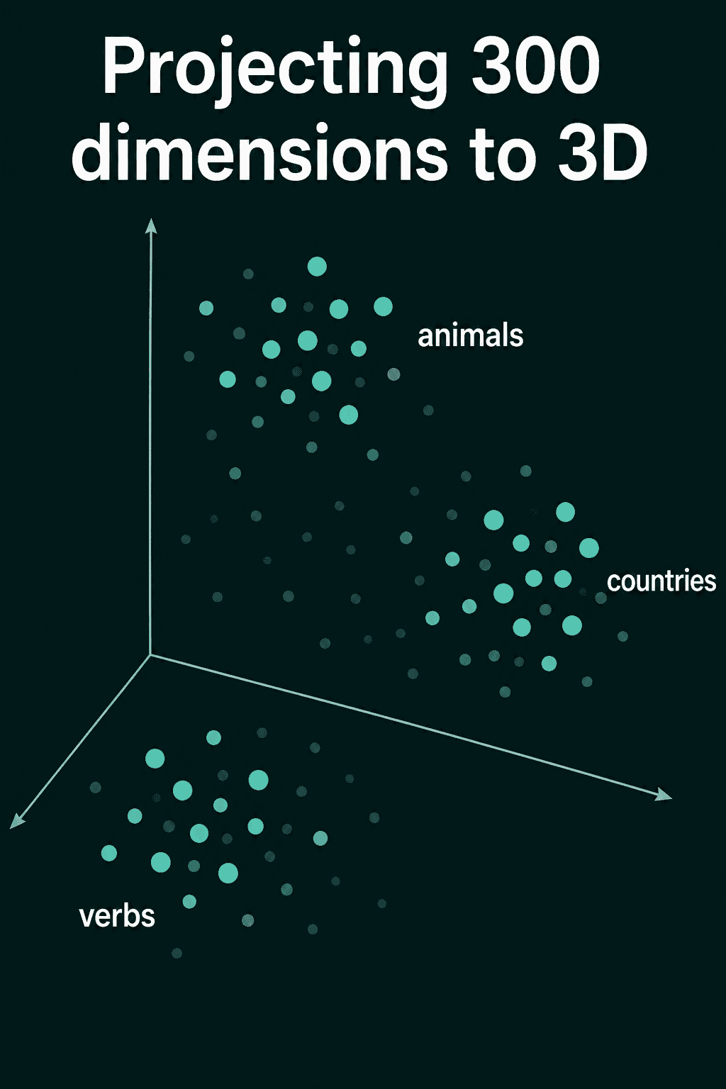
Two dimensions is the common choice because it fits flat on a page. Three dimensions keep one more axis of structure, at the cost of a plot you have to rotate.
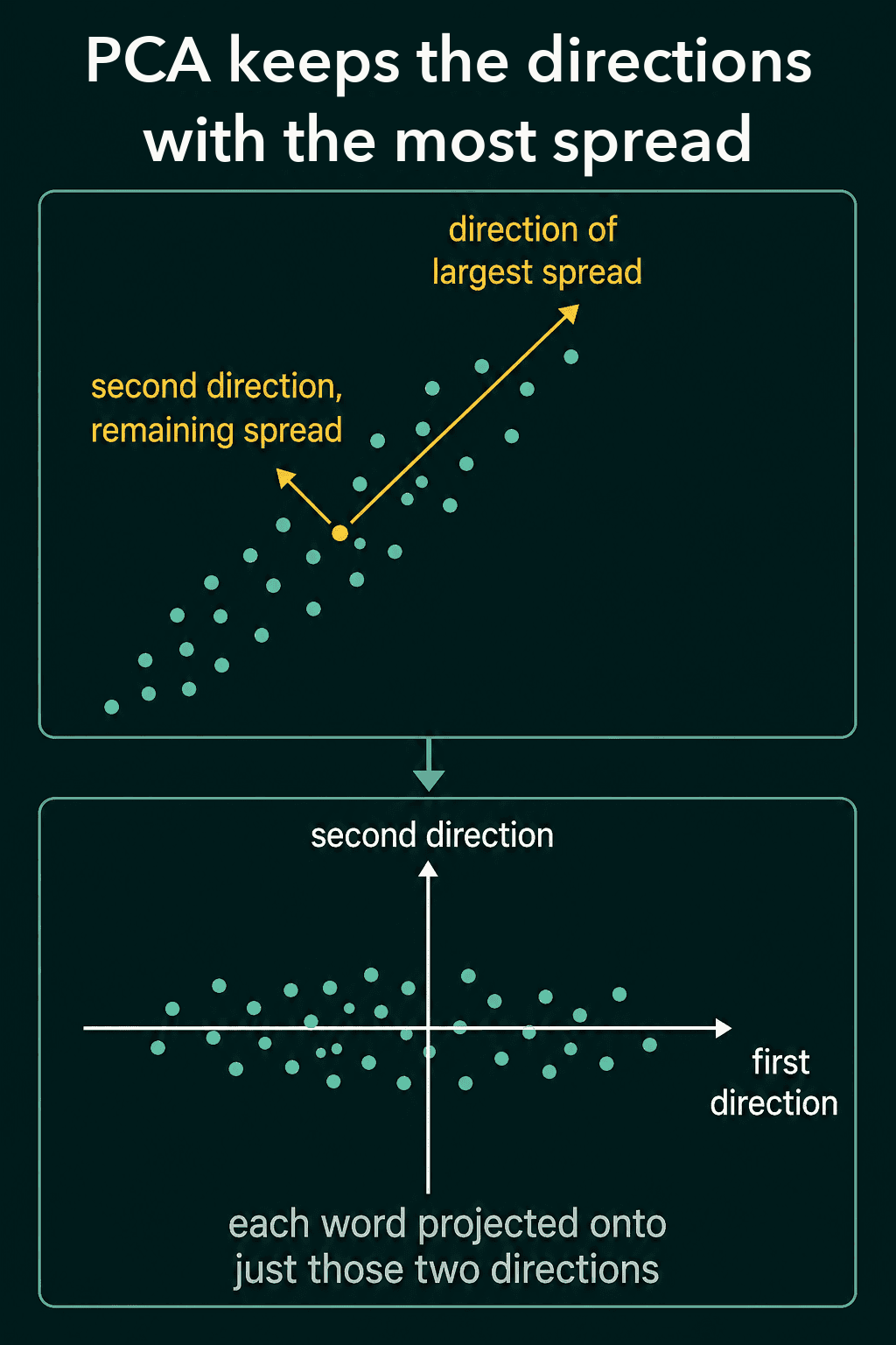
PCA: keep the directions with the most spread
PCA, short for principal component analysis, is one way to do the reduction. Imagine all the word vectors as a cloud of points. PCA finds the direction through that cloud along which the points are spread out the most, which is called the direction of largest variance. Then it finds a second direction, at a right angle to the first, along which the remaining spread is largest. For a 2D plot those two directions become the x and y axes, and each word's 300 numbers are projected onto them to give its point.
The code below builds 9 made-up word vectors with 50 numbers each, in three groups, so the results are easy to check. Real embeddings come from training, and the steps are the same.
1import torch
2
3torch.manual_seed(0)
4words = ["cat", "dog", "horse", "paris", "berlin", "rome", "red", "blue", "green"]
5centers = torch.randn(3, 50) * 2
6groups = torch.tensor([0, 0, 0, 1, 1, 1, 2, 2, 2])
7emb = centers[groups] + torch.randn(9, 50)
8
9# PCA: center the vectors, then keep the two directions of largest spread
10centered = emb - emb.mean(dim=0)
11U, S, Vt = torch.linalg.svd(centered, full_matrices=False)
12points = centered @ Vt[:2].T          # shape (9, 2): one x, y per word
13for w, (x, y) in zip(words, points.tolist()):
14 print(f"{w:7s} {x:6.1f} {y:6.1f}")1cat -11.1 -8.9
2dog -9.4 -6.9
3horse -9.5 -8.8
4paris 12.2 -3.0
5berlin 13.9 -3.7
6rome 12.3 -4.5
7red -2.1 12.7
8blue -0.8 10.4
9green -5.5 12.6The animals land near $(-10, -8)$, the cities near $(13, -4)$ and the colors near $(-3, 12)$. torch.linalg.svd returns the directions of largest spread as the rows of Vt, first one first.
Because PCA keeps the directions with the most spread, it tends to preserve the large-scale picture of which words are broadly similar to which. It has nothing aimed at keeping small, tight groups together when they do not line up with those top directions.
t-SNE: keep each word's neighbors together
t-SNE works on local neighborhoods instead. First it measures, for every pair of words, how likely one is to be a neighbor of the other in the original 300 dimensions. Close words get a high probability and far words get a low one. Then it places every word at a random point in 2D and moves the points a little at a time, over many steps, until the same neighbor probabilities hold in the 2D layout. Words that were close get pulled together and words that were far apart get pushed apart.
So tight groups in the original space tend to stay tight on a t-SNE plot. The distances between groups are not kept. Two groups that land far apart on a t-SNE plot are not necessarily far apart in the real embedding.
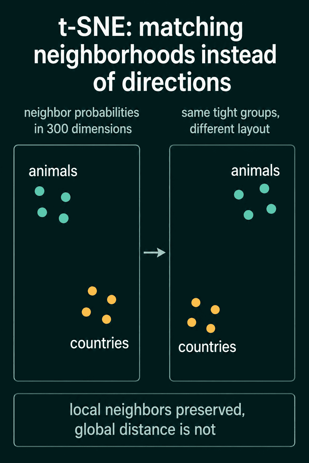
UMAP solves a similar problem to t-SNE with different math. It also keeps nearby points near each other, and it is usually faster on large vocabularies.
Nearest neighbors: which words sit closest to one word?
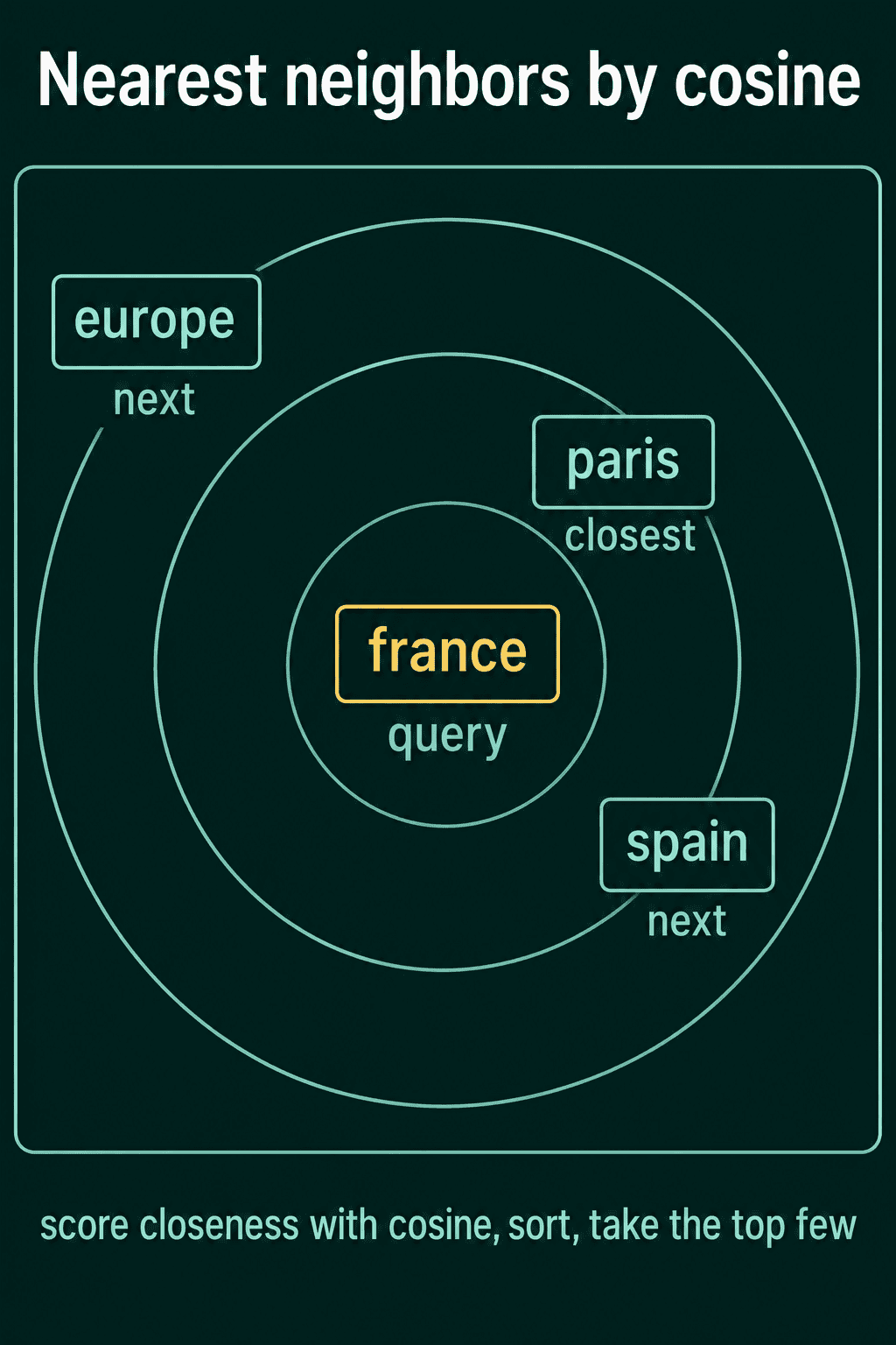
A plot is one way to inspect vectors. You can also compare two vectors directly by how close they are, without making a picture first. Close vectors usually mean similar words.
The usual closeness score for embeddings is cosine similarity, which compares the directions of two vectors: 1 when they point the same way, 0 at a right angle and -1 when they point in opposite directions. The cosine similarity post works through it by hand.
To find a word's nearest neighbors, score it against every other word, sort and keep the top few:
1import torch
2import torch.nn.functional as F
3
4torch.manual_seed(0)
5words = ["cat", "dog", "horse", "paris", "berlin", "rome", "red", "blue", "green"]
6centers = torch.randn(3, 50) * 2
7groups = torch.tensor([0, 0, 0, 1, 1, 1, 2, 2, 2])
8emb = centers[groups] + torch.randn(9, 50)
9
10def nearest_neighbors(query, embeddings, k):
11    sims = F.cosine_similarity(query.unsqueeze(0), embeddings)
12    top = sims.topk(k + 1).indices
13    return top[1:]  # drop the word itself
14
15i = words.index("paris")
16print([words[j] for j in nearest_neighbors(emb[i], emb, 2)])1['rome', 'berlin']The function asks for $k + 1$ results and drops the first, because the closest vector to any word is the word itself. On a real trained embedding, the neighbors of france tend to be words like paris, spain and europe.
Clustering: which words form groups?
Nearest neighbors answers a question about one word. Clustering asks it for the whole vocabulary at once: which words fall into the same group? It works from the distances between the full vectors, not from a plot.
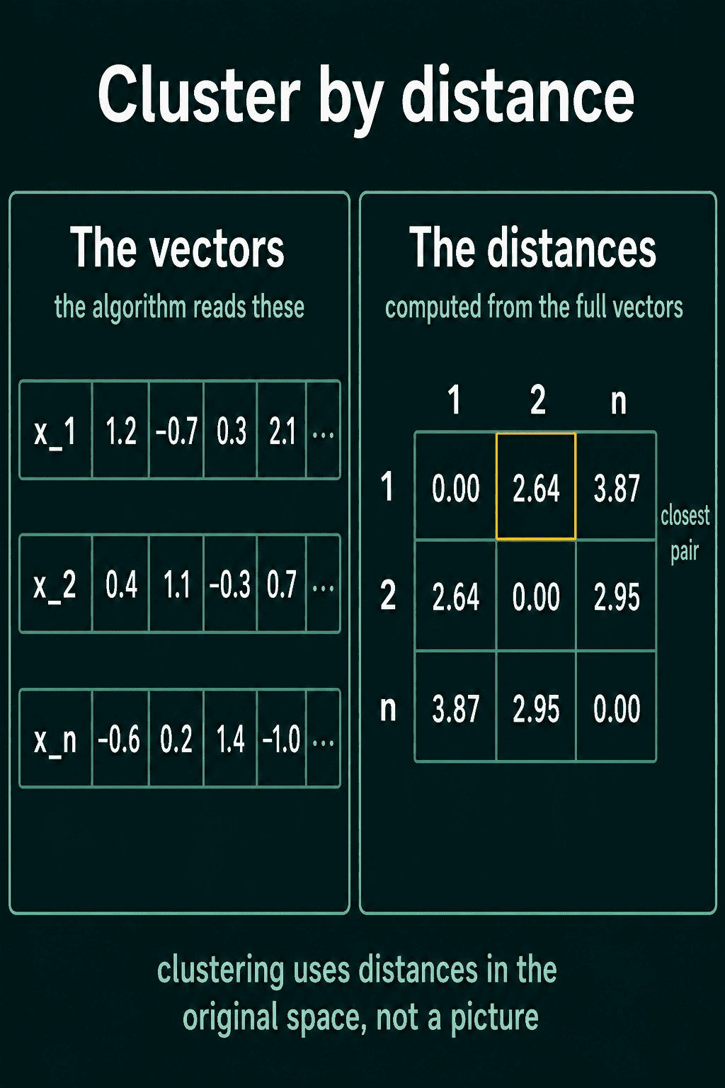
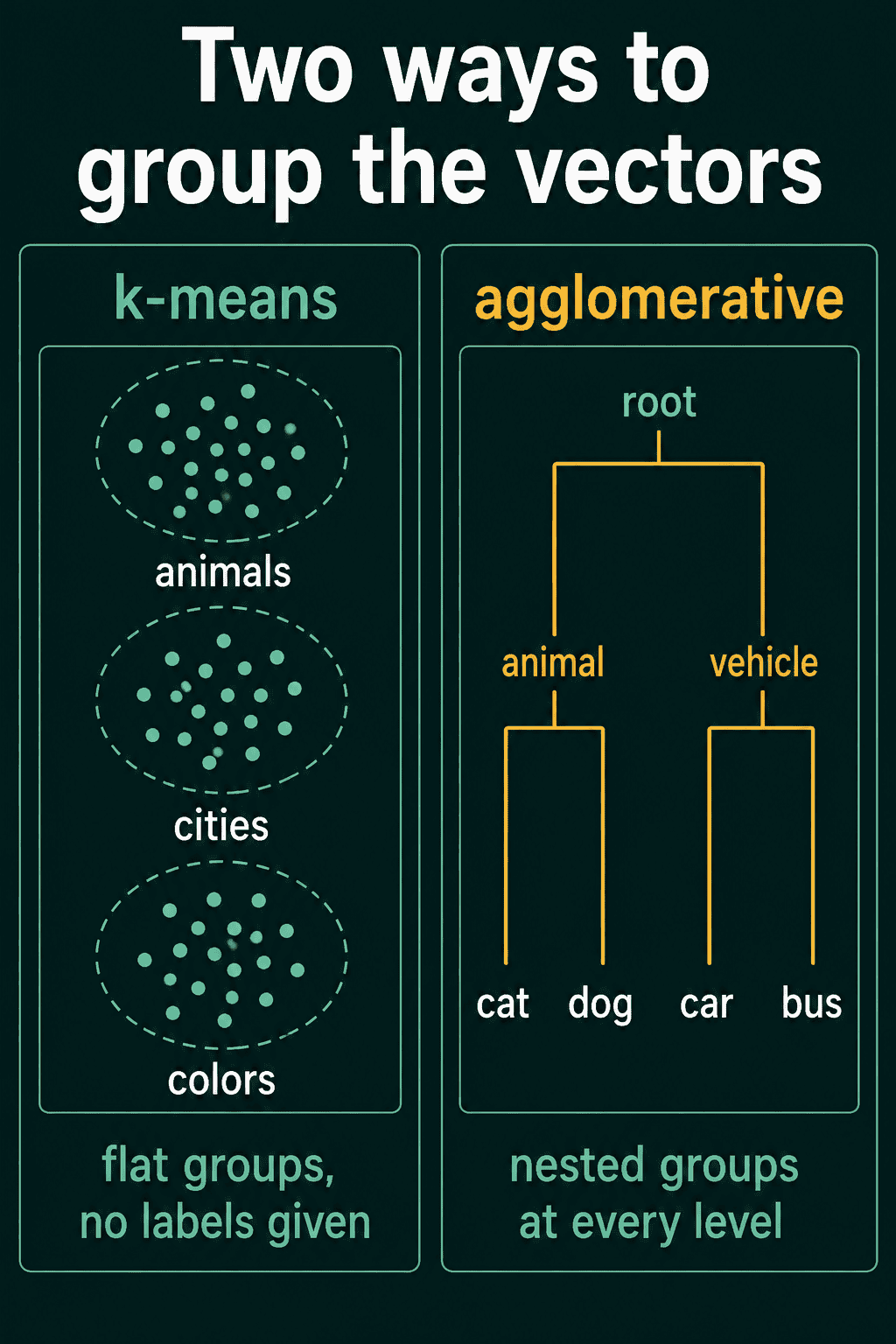
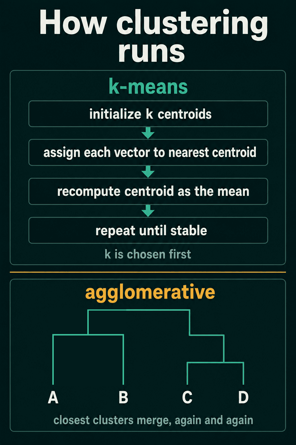
K-means is the most common method. You choose the number of groups $k$ first, because k-means does not discover it. Then it repeats two steps: assign every vector to its nearest centroid (the center point of a group), and move each centroid to the average of the vectors assigned to it. It stops when the assignments no longer change.
1import torch
2
3torch.manual_seed(0)
4words = ["cat", "dog", "horse", "paris", "berlin", "rome", "red", "blue", "green"]
5centers = torch.randn(3, 50) * 2
6groups = torch.tensor([0, 0, 0, 1, 1, 1, 2, 2, 2])
7emb = centers[groups] + torch.randn(9, 50)
8
9def kmeans(x, k, steps=20):
10    centroids = x[torch.randperm(len(x))[:k]]          # k random words as the starting centroids
11    for _ in range(steps):
12        assign = torch.cdist(x, centroids).argmin(dim=1)  # nearest centroid for each vector
13        centroids = torch.stack([x[assign == c].mean(dim=0) for c in range(k)])
14    return assign
15
16assign = kmeans(emb, k=3)
17for c in range(3):
18 print(c, [w for w, a in zip(words, assign.tolist()) if a == c])10 ['paris', 'berlin', 'rome']
21 ['red', 'blue', 'green']
32 ['cat', 'dog', 'horse']Nobody told k-means which words are cities. The groups come from the distances alone, and on real embeddings k-means tends to recover groups like animals, cities and colors in the same way. The result is a flat split where every word lands in exactly one group. Different starting centroids can give different final groups, so real runs usually try several starts.
Agglomerative clustering starts from the other end. Every word begins as its own group. Then the two closest groups merge again and again until one tree remains. A linkage rule says what "closest groups" means: average linkage uses the average distance between their members, and complete linkage uses the farthest pair. The tree holds groups at several levels at once, so cat and dog sit together inside a wider animal group, and you choose how coarse a grouping to read off.
How do you know if embeddings are good?
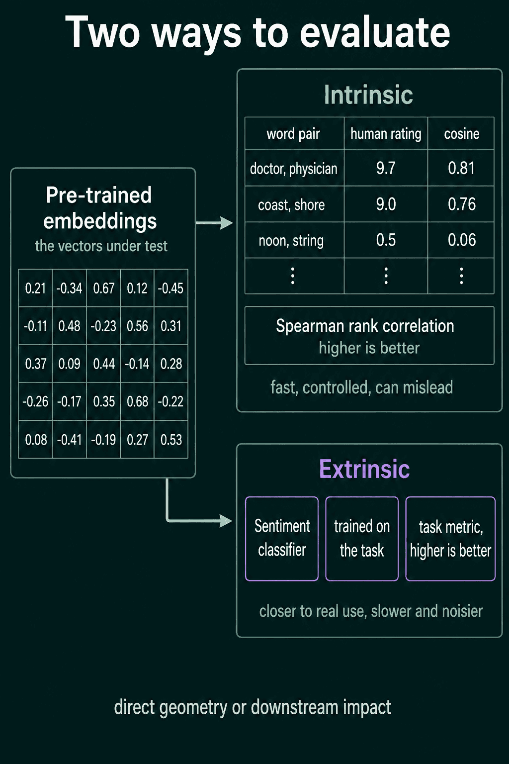
There are two ways to judge a set of embeddings. Intrinsic evaluation checks the vectors on their own, by testing whether their geometry agrees with human judgments about meaning. Extrinsic evaluation plugs them into a real task and checks whether the task gets better. The first is fast and controlled but can mislead. The second is closer to real use, but slower, noisier and tied to the task you picked.
Intrinsic evaluation: compare with human judgments
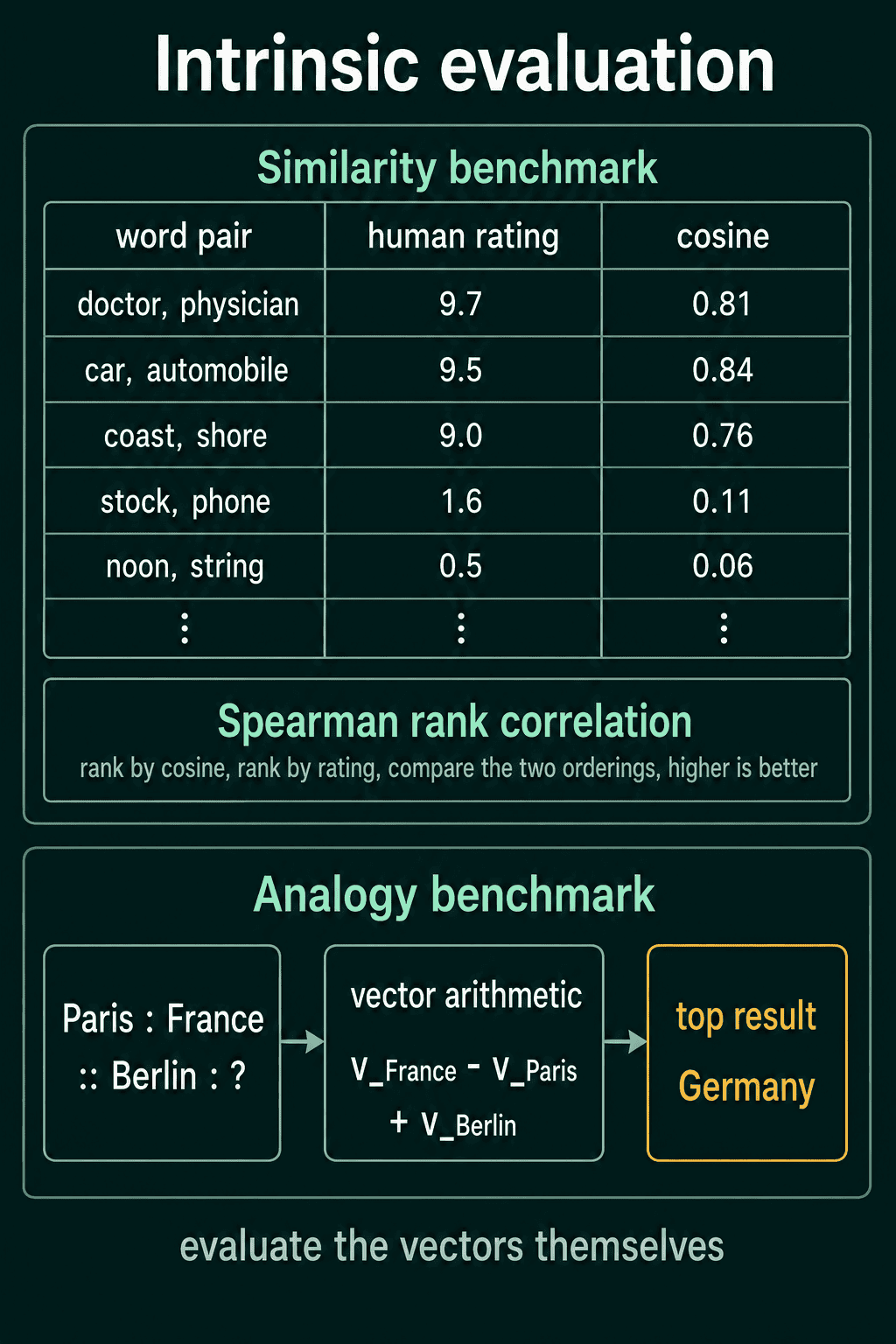
A similarity benchmark is a list of word pairs that people rated for how similar they are. You compute the cosine similarity of each pair from your embeddings and check whether the two orderings agree. The usual score is Spearman rank correlation: rank the pairs by your cosine score, rank them again by the human rating, and measure how well the two rankings match on a scale from -1 to 1.
For example, take five rated pairs:
| Pair | Human rating | Cosine |
|---|---|---|
| doctor, physician | 9.7 |
0.81 |
| car, automobile | 9.5 |
0.84 |
| coast, shore | 9.0 |
0.76 |
| stock, phone | 1.6 |
0.11 |
| noon, string | 0.5 |
0.06 |
Both orderings put the pair noon and string lowest, then stock and phone, then coast and shore. They disagree only on the top two. People rate doctor and physician higher, and the embeddings score car and automobile higher. That one swap brings the score down from 1 to 0.9:
1import torch
2
3human = torch.tensor([9.7, 9.5, 9.0, 1.6, 0.5])       # doctor-physician, car-automobile, coast-shore, stock-phone, noon-string
4cosine = torch.tensor([0.81, 0.84, 0.76, 0.11, 0.06])
5
6def ranks(x):
7    return x.argsort().argsort().float()             # 0 for the smallest value, 1 for the next, ...
8
9def spearman(a, b):
10    ra, rb = ranks(a), ranks(b)
11    ra, rb = ra - ra.mean(), rb - rb.mean()
12    return (ra * rb).sum() / (ra.norm() * rb.norm())
13
14print(round(spearman(human, cosine).item(), 2))10.9An analogy benchmark tests a different property. It holds questions like "Paris is to France as Berlin is to what?" and checks whether vector arithmetic finds the answer. Take the vector for France, subtract Paris and add Berlin, then look up the nearest word. A good embedding returns Germany.
Some datasets use other formats, such as picking the closest synonym from a list, or rating how similar two words are inside a given sentence.
Similarity is not the same as relatedness
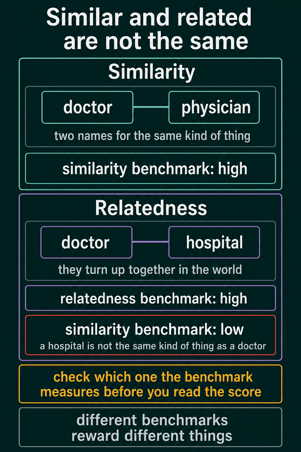
Different benchmarks measure different things, and mixing them up is a common trap. A similarity benchmark rates true similarity, so doctor and physician score high because they are two names for the same kind of thing, and doctor and hospital score low. A relatedness benchmark also credits words that turn up together in the world, so doctor and hospital score high there even though a hospital is not like a doctor. Read a benchmark's documentation to see which one it rates before reading your score.
Two more cautions apply. A strong intrinsic score does not promise that the embeddings help on a real task. And embeddings shift a little from one training run to the next, because training starts from random numbers, so one score from one run is shaky. Train several and average before you trust a number.
Extrinsic evaluation: plug them into a task
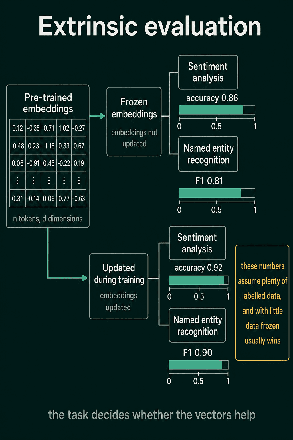
Extrinsic evaluation skips the geometry and asks whether the embeddings make a real system better. You use them as the input to a model for a task you care about and measure that task's score. Sentiment classification (is a review positive or negative?) is scored by accuracy. Named entity recognition means finding the names of people, places and organizations in text. It is often scored by F1, a number between 0 and 1 that combines how many names the model found with how many of its answers were right. Better embeddings should lift the score.
This is the closest test to real use. It is also slower than a similarity benchmark and noisier, and it is tied to one task, so a win on sentiment does not guarantee a win on named entity recognition.
One more choice comes up here. You can freeze the embeddings, which keeps them fixed while the task model trains, or let the task model update them during training. Updating them helps when you have plenty of labeled data. With little data, frozen embeddings are usually safer.
Common mistakes
- Reading distances between groups on a t-SNE plot. t-SNE keeps neighbors together and does not keep the gaps between groups.
- Keeping the query word in its own neighbor list. The top match for any word is the word itself, so ask for $k + 1$ and drop the first.
- Trusting one k-means run. The result depends on the starting centroids and on the $k$ you chose. Try several starts and a few values of $k$.
- Scoring on the wrong kind of benchmark. A relatedness score says little about similarity, and the reverse holds too.
- Picking embeddings from one intrinsic score. Average over several training runs, then confirm on the task you care about.
Related concepts
The word embeddings post covers where the vectors come from and how a lookup table stores them, and the Word2Vec vs GloVe vs fastText post compares three ways to train them. Every method in this post scores one vector per word, which is the limit covered in the static vs contextual embeddings post.
QuiddityML teaches visualizing, clustering and evaluating embeddings as separate concepts in the word representations unit of its NLP track. The exercises include writing the nearest neighbors function from scratch, putting the k-means loop in order and spotting the bug in a neighbor search (QuiddityML).