By Sagi Shaier · 31 October 2026 · 7 min read
Negative sampling and hierarchical softmax explained
Why training skip-gram with a full softmax gets slow on a large vocabulary, and how each shortcut replaces it, with worked numbers and short PyTorch code for both.
Negative sampling and hierarchical softmax are two ways to train Word2Vec without comparing every training example against every word in the vocabulary. Word2Vec learns word vectors by predicting which words appear near each other, and on a large vocabulary that prediction is too slow to run across a big collection of text. Each method swaps the slow step for a small number of yes-or-no decisions.
What makes the full softmax slow?
The skip-gram version of Word2Vec takes a center word and predicts one word near it. Each word has two vectors: an input vector $\mathbf{v}$ and an output vector $\mathbf{v}'$. The score for a pair of words is the dot product of the two, which multiplies matching entries and adds them up. Softmax then turns scores into a probability for the context word $w$:
$$P(w \mid c) = \frac{\exp(\mathbf{v}'^{\top}_{w} \mathbf{h})}{\sum_{w'=1}^{V} \exp(\mathbf{v}'^{\top}_{w'} \mathbf{h})}$$
Here $\mathbf{h}$ is the input word's vector and $V$ is the vocabulary size. The bottom of the fraction runs over every word in the vocabulary.
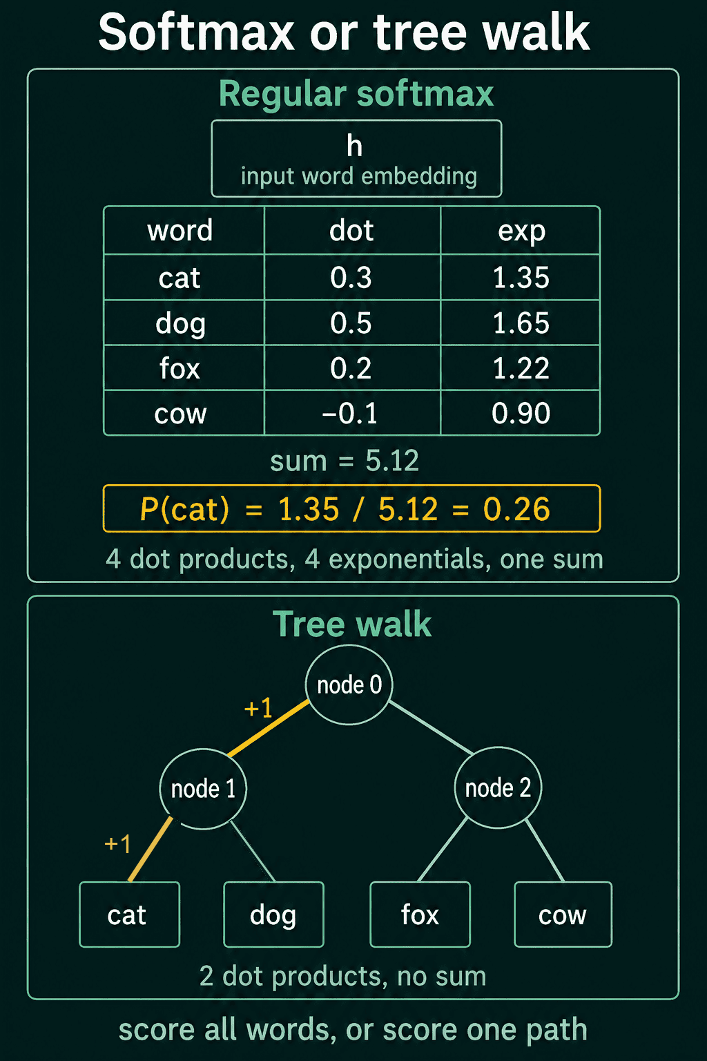
Take a vocabulary of four words: cat, dog, fox and cow. Say their dot products with $\mathbf{h}$ are 0.3, 0.5, 0.2 and -0.1. Raising $e$ to each gives 1.35, 1.65, 1.22 and 0.90. Those add up to 5.12, so the probability of cat is:
$$P(\text{cat} \mid c) = 1.35 / 5.12 \approx 0.26$$
Scoring one word touched all 4 words. With a vocabulary of a million words, that is a million dot products for each training pair, which is far too slow on a large text.
How negative sampling works
Negative sampling replaces the question "which of the million words is the context word?" with a cheaper one: "is this pair of words real, or was it made up?"
Each true center and context pair is joined by a few random words called negatives, and the model learns to tell the true pair from the fake ones. The center word is checked against a handful of words and the rest of the vocabulary is left alone.
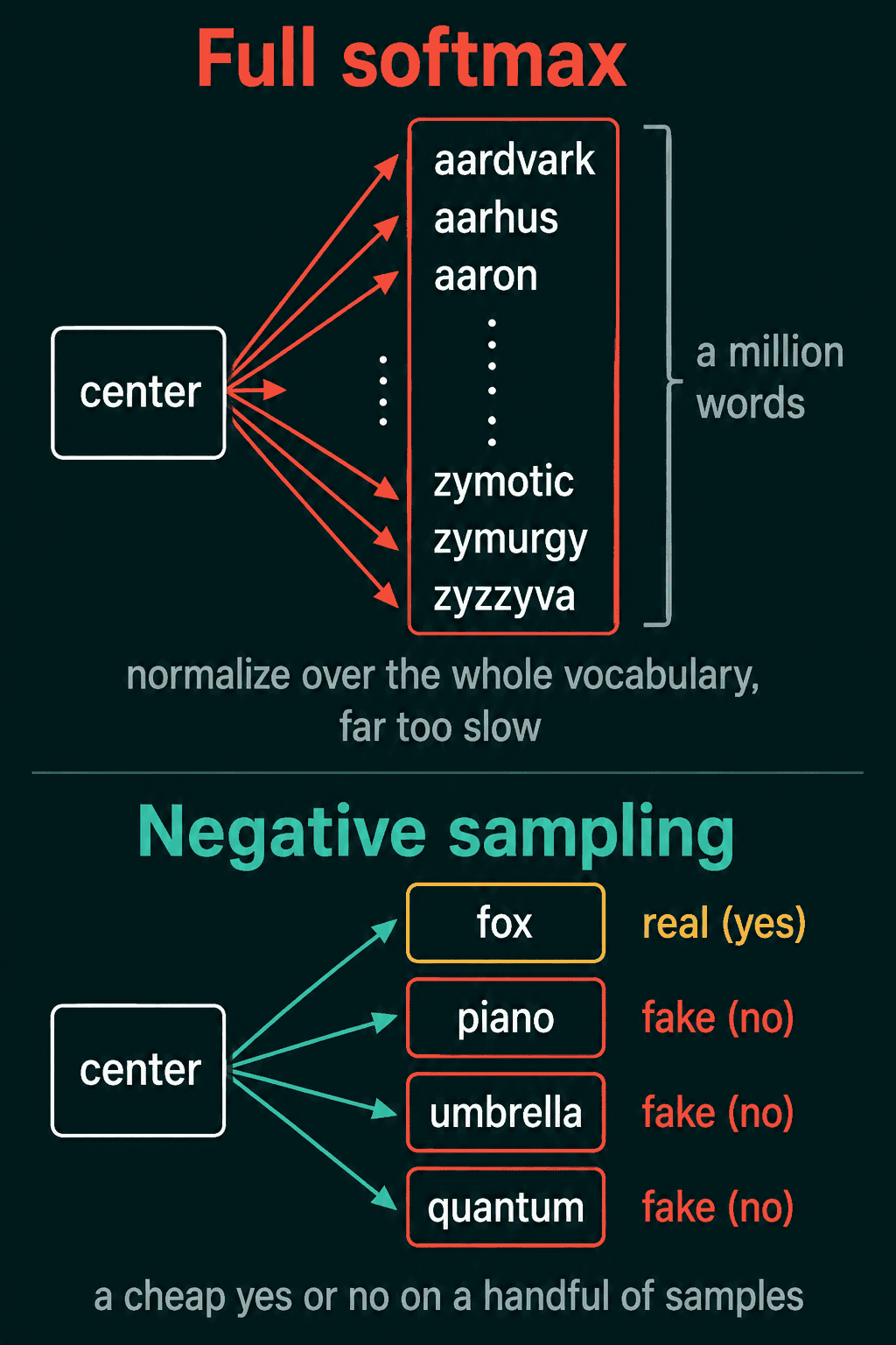
The yes-or-no answer comes from the sigmoid function, which squashes any real number into the range 0 to 1:
$$\sigma(x) = \frac{1}{1 + e^{-x}}$$
A dot product of 2.5 gives $\sigma(2.5) = 0.92$, close to yes. A dot product of -1 gives $\sigma(-1) = 0.27$, closer to no. The sigmoid also has the property that $\sigma(-x) = 1 - \sigma(x)$, and you can check that here: $\sigma(1) = 0.73$, which is $1 - 0.27$. So putting a minus sign in front of a negative's dot product asks for its score to be pushed down.
Write $w_I$ for the center word, $w_O$ for the true context word and $n_k$ for the $k$-th negative. Training maximizes:
$$\log \sigma(\mathbf{v}'^{\top}_{w_O} \mathbf{v}_{w_I}) + \sum_{k} \log \sigma(-\,\mathbf{v}'^{\top}_{n_k} \mathbf{v}_{w_I})$$
The first term pushes the true pair's sigmoid toward 1. The sum pushes each negative's sigmoid toward 0.
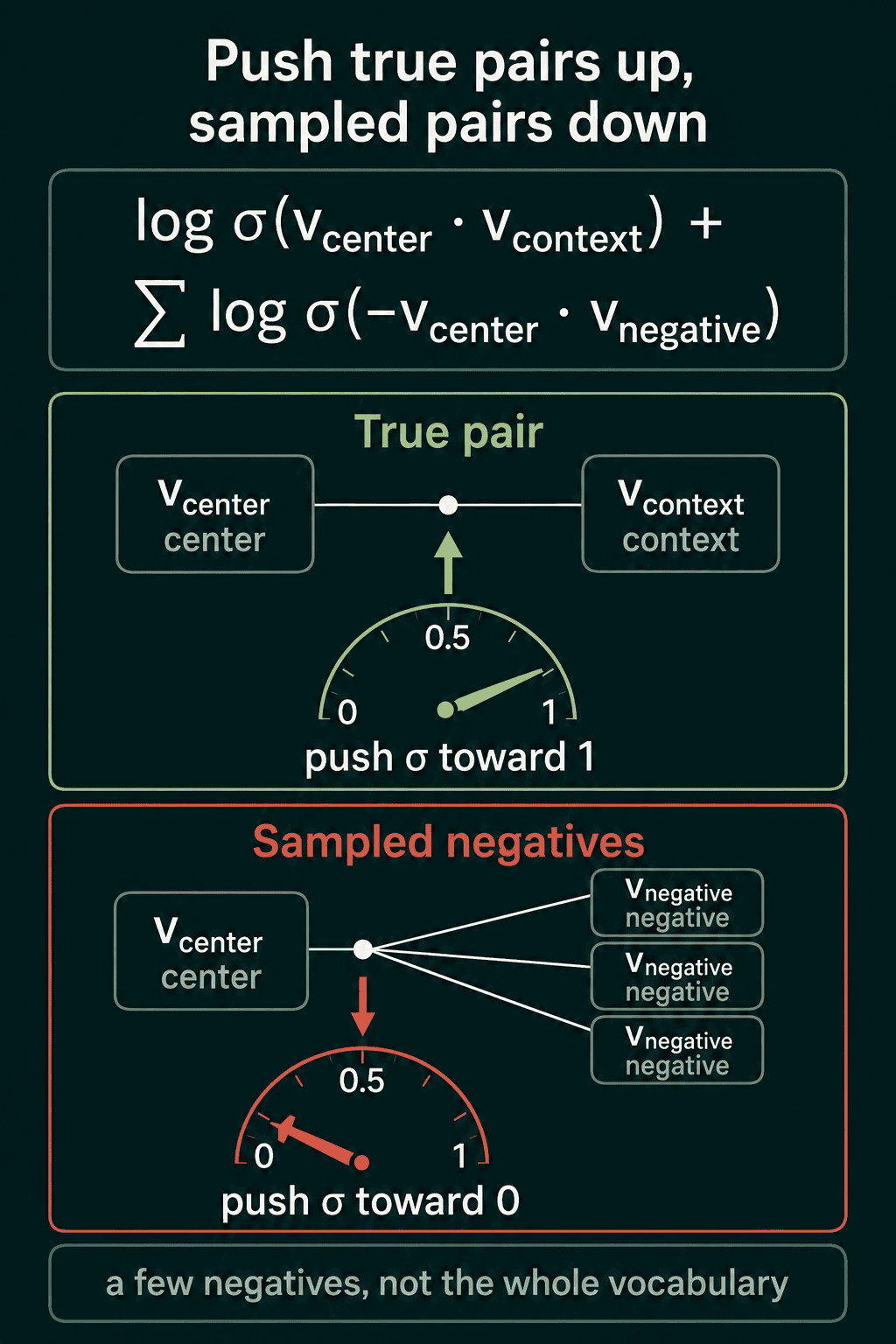
Here is that sum with real numbers. Say the center vector is $[1, 0.5]$ and the true context vector is $[2, 1]$, so their dot product is 2.5. Two negatives have vectors $[-1, 0]$ and $[0.5, -1]$, which give dot products of -1 and 0. The three terms are $\log \sigma(2.5) = -0.079$, $\log \sigma(1) = -0.313$ and $\log \sigma(0) = -0.693$. They add up to -1.085, and the loss is the negative of that:
1import torch
2
3def neg_sampling_loss(v_center, v_context, v_negatives):
4    pos = torch.log(torch.sigmoid(v_context @ v_center))
5    neg_scores = -(v_negatives @ v_center)
6    neg = torch.log(torch.sigmoid(neg_scores)).sum()
7    return -(pos + neg)
8
9v_center = torch.tensor([1.0, 0.5])
10v_context = torch.tensor([2.0, 1.0])
11v_negatives = torch.tensor([[-1.0, 0.0], [0.5, -1.0]])
12
13print(neg_sampling_loss(v_center, v_context, v_negatives))
It prints:
1tensor(1.0853)Each row of v_negatives is one sampled word, and @ is the dot product. Every training step touches the center word, one true context word and a few negatives, however large the vocabulary is.
Where do the negatives come from?
The negatives are not drawn evenly from the vocabulary. They come from the unigram distribution, which is how often each word appears in the text, raised to the power 0.75:
1counts = torch.tensor([600.0, 200.0, 120.0, 60.0, 20.0])
2
3print(counts / counts.sum())
4
5freqs = counts ** 0.75
6probs = freqs / freqs.sum()
7print(probs)
8
9torch.manual_seed(0)
10print(torch.multinomial(probs, num_samples=5, replacement=True))
It prints:
1tensor([0.6000, 0.2000, 0.1200, 0.0600, 0.0200])
2tensor([0.5016, 0.2200, 0.1500, 0.0892, 0.0391])
3tensor([4, 1, 0, 3, 1])
Raising the counts to three-quarters flattens them. The most common word drops from 0.60 to 0.50, and the rarest doubles from 0.02 to 0.04. So rare words show up as negatives more often than their raw frequency would allow. The last line draws five negatives from those probabilities, each printed as a position in the vocabulary.
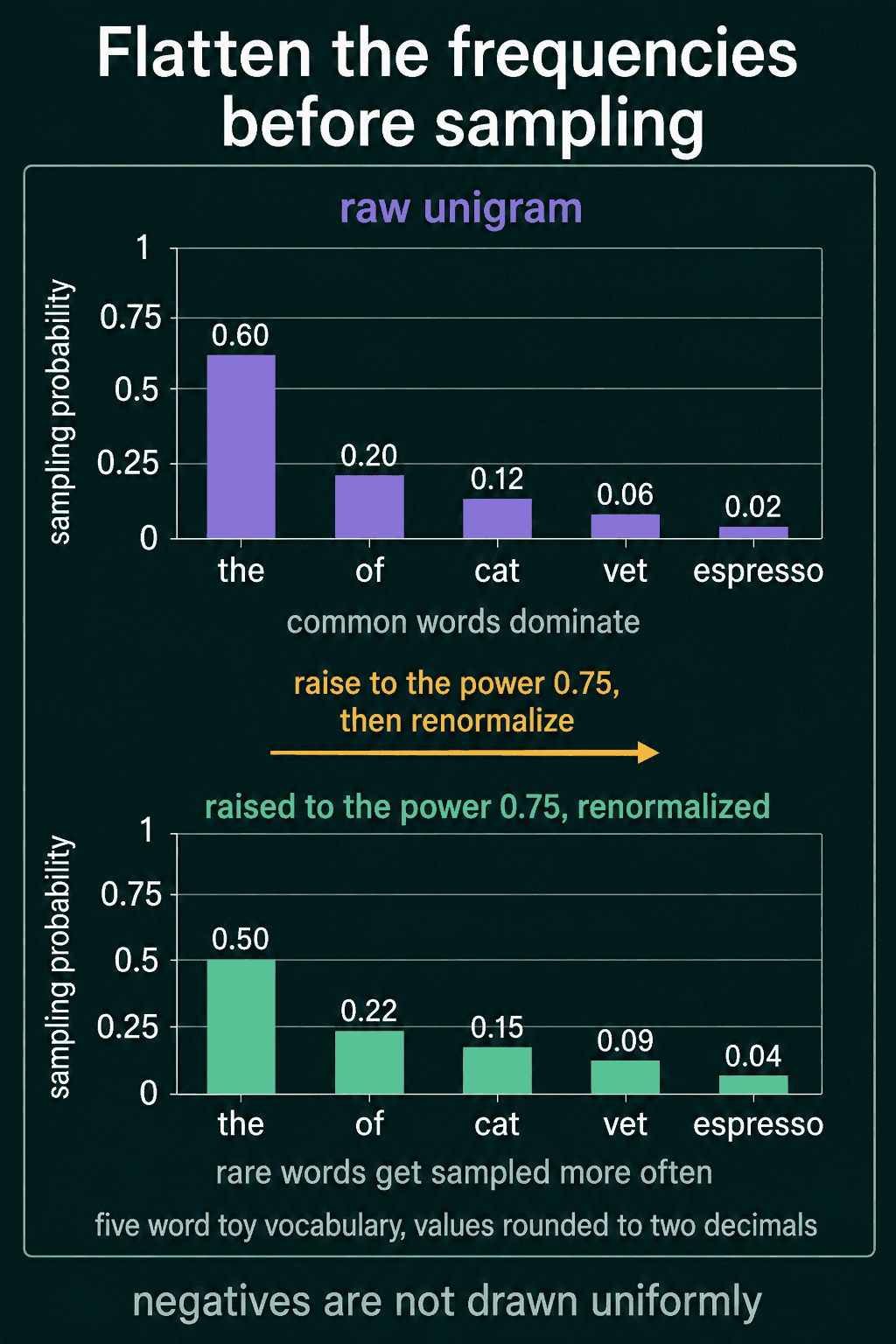
The power 0.75 is a common default for Word2Vec training. As for how many negatives to draw, around 5 to 20 per true pair is typical for small texts and 2 to 5 for large ones.
How hierarchical softmax works
Hierarchical softmax takes another route. Arrange the whole vocabulary as the leaves of a binary tree, where each split has a left and a right branch. To score a word, walk the path from the root down to that word's leaf and make one binary decision at each node. The word's probability is the product of those decisions:
$$P(w \mid c) = \prod_{j=1}^{L(w)-1} \sigma\big(s_j \cdot \mathbf{v}_{n(w,j)}^\top \mathbf{h}\big)$$
$\mathbf{h}$ is the input word's vector. $n(w,j)$ is the $j$-th node on the path to $w$, and $L(w)$ is the number of nodes on that path counting the leaf. Every inner node has its own learned vector $\mathbf{v}_{n(w,j)}$, and the leaves have no vector. $s_j$ is $+1$ if the path goes left at that node and $-1$ if it goes right.
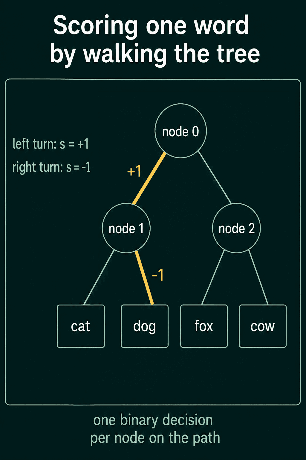
Reaching "dog" in this tree means going left at node 0 and right at node 1, so the path is [0, 1] and the signs are [1, -1]. The formula turns into a short loop over that path:
1def hierarchical_softmax_prob(h, node_vecs, path, signs):
2    prob = 1.0
3    for node, s in zip(path, signs):
4        score = s * (node_vecs[node] @ h)
5        prob = prob * torch.sigmoid(score)
6    return prob
7
8h = torch.tensor([1.0, 0.0])
9node_vecs = torch.tensor([[0.5, 0.5], [2.0, -1.0], [0.0, 1.0]])
10
11paths = {
12    "cat": ([0, 1], [1, 1]),
13    "dog": ([0, 1], [1, -1]),
14    "fox": ([0, 2], [-1, 1]),
15    "cow": ([0, 2], [-1, -1]),
16}
17
18total = 0.0
19for word, (path, signs) in paths.items():
20    prob = hierarchical_softmax_prob(h, node_vecs, path, signs)
21    total += prob
22    print(word, round(prob.item(), 4))
23print(round(total.item(), 4))
It prints:
1cat 0.5483
2dog 0.0742
3fox 0.1888
4cow 0.1888
51.0
prob starts at 1.0 because every step multiplies a new factor into it. Each loop computes one signed dot product, turns it into a probability with the sigmoid, and multiplies that in.
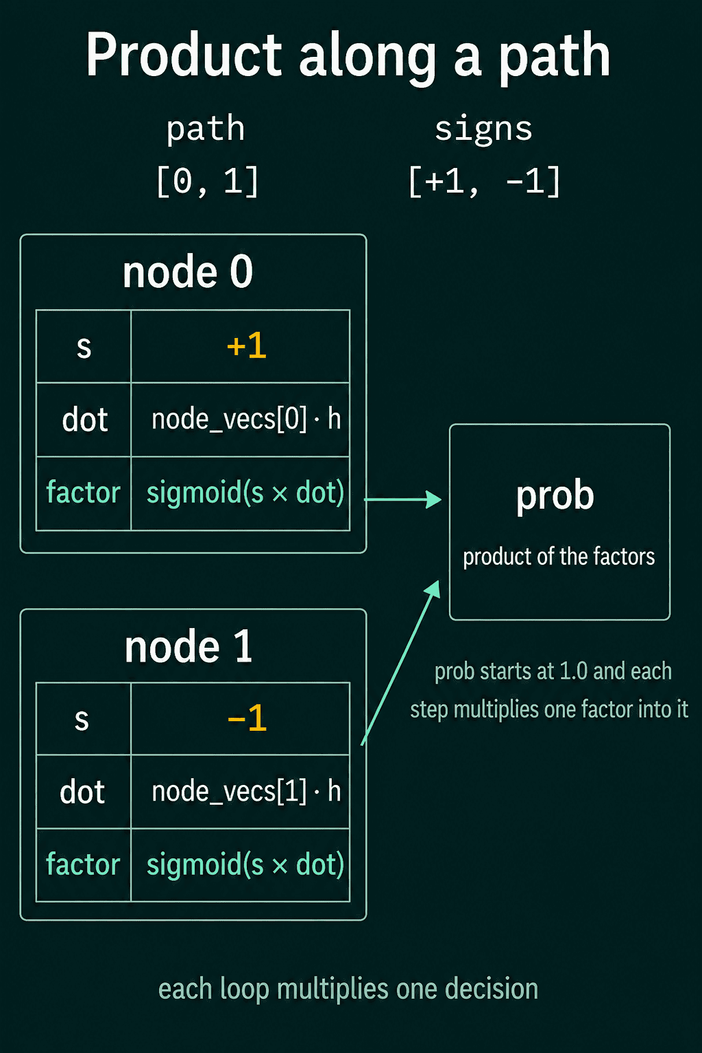
The numbers for "dog" are short enough to do by hand. At node 0 the dot product is $0.5 \times 1.0 + 0.5 \times 0.0 = 0.5$, the sign is $+1$, and $\sigma(0.5) = 0.62$. At node 1 the dot product is $2.0$, the sign is $-1$, and $\sigma(-2.0) = 0.12$. The product is $0.62 \times 0.12 = 0.07$, which matches the 0.0742 above after rounding.
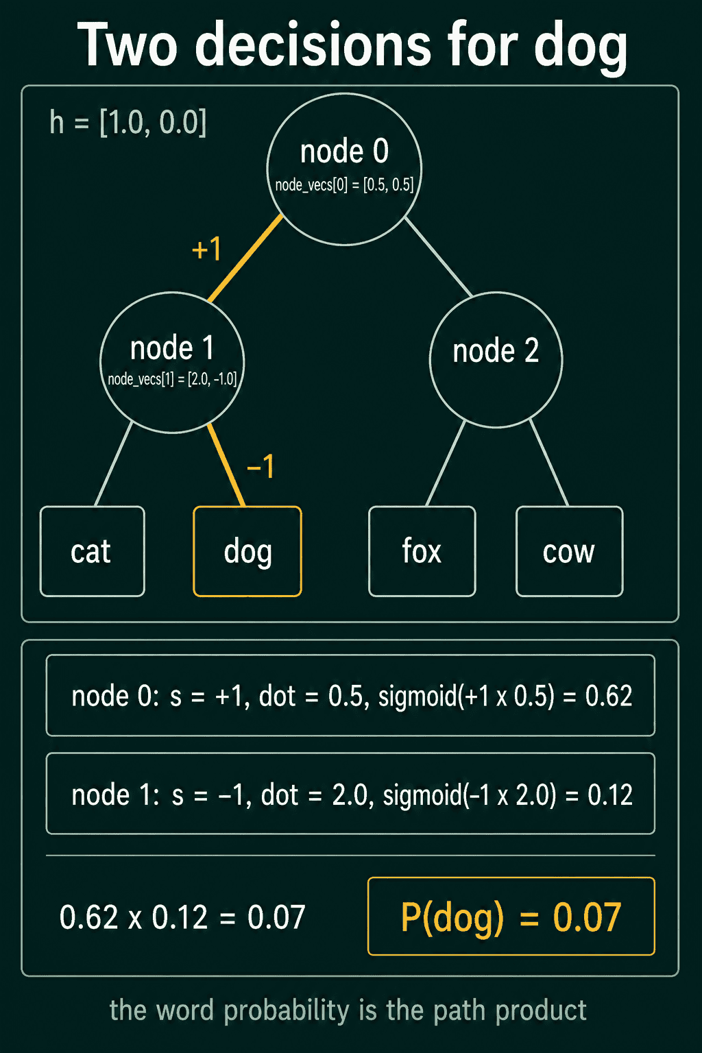
The four probabilities in that output add up to 1. The signs are the reason: at any node, the left branch gets $\sigma(x)$ and the right branch gets $\sigma(-x)$, and those two add up to 1. These node vectors are toy numbers chosen for the arithmetic, so the results are not meant to match a full softmax over the same four words.
A balanced tree has a depth of about $\log_2 V$. For a million words, that is:
$$\log_2 1{,}000{,}000 \approx 20$$
So one training pair takes about 20 binary decisions instead of a million dot products. A common choice is a Huffman tree, which puts frequent words on shorter paths, so the words you score most often are the cheapest.
Negative sampling vs hierarchical softmax
| Method | Work per pair, 1M words | Output side stores |
|---|---|---|
| Full softmax | 1,000,000 dot products | one vector per word |
| Negative sampling | 1 + number of negatives | one vector per word |
| Hierarchical softmax | about 20 sigmoid decisions | one vector per inner node |
Both shortcuts are training options, so the input embedding table you keep at the end is the same kind of object either way. Negative sampling is the simpler one to write, because it needs no tree. It does need a list of word counts to draw negatives from. Hierarchical softmax needs a tree built up front and gives you a probability that sums to 1 across the vocabulary. On a small vocabulary, the full softmax is fine, since the sum is short.
Common mistakes
- Dropping the minus sign on the negatives. Without it, the loss pushes fake pairs up along with the real one. In the code, that sign lives in
neg_scores = -(v_negatives @ v_center). - Drawing negatives evenly. Sampling every word with the same chance makes rare words far too common as negatives. Use the counts raised to 0.75.
- Mixing up the signs on a path.
signsmust line up withpath, one sign per node. A flipped sign scores the sibling leaf instead of the word you meant.
Related concepts
The skip-gram and CBOW post builds the full-softmax model these shortcuts replace. fastText trains with the same negative sampling objective, and GloVe fits word pair counts with no sampling. In the word embeddings post, you can see what the resulting table holds.
QuiddityML teaches negative sampling and hierarchical softmax as two concepts in the word representations unit of its NLP track, and the exercises include turning the negative sampling objective into code and tracing the tree walk for one word (QuiddityML).