By Sagi Shaier · 10 October 2026 · 5 min read

Broadcasting in NumPy and PyTorch explained

How to tell in advance whether two shapes can be combined and what shape comes out, how to make a vector stretch across rows or across columns, and how to build a table of every pairwise difference without a loop, with PyTorch code for each.

Broadcasting is the set of rules NumPy and PyTorch use to combine two arrays of different shapes in an elementwise operation, by stretching size-1 axes to match without copying any data. It is what lets x + bias add one bias vector to every row of a batch, and it is behind a common kind of silent shape bug.

The problem broadcasting solves

An elementwise operation combines two arrays position by position: addition, subtraction, the elementwise product *, and comparisons like >. On its own that requires both arrays to have exactly the same shape.

In model code the shapes often differ. A batch x of 32 examples with 4 features each has shape $(32, 4)$, and a bias vector with one number per feature has shape $(4,)$. Adding the bias to every row by hand would mean copying it 32 times into a $(32, 4)$ array first. Broadcasting does that matching automatically and without the copy.

The rule

Line the two shapes up from the right, and compare them one axis at a time. Two sizes are compatible if they are equal, or if one of them is 1. A size-1 axis is stretched to match the other size, conceptually only: the numbers are reused, not copied in memory. If one shape has fewer axes, it is treated as having extra size-1 axes on the left.

For x + bias, $(4,)$ is treated as $(1, 4)$ and compared with $(32, 4)$. The right axes are both 4, and the left axes are 32 and 1, so the 1 stretches to 32 and the result has shape $(32, 4)$, with the same bias added to every row.

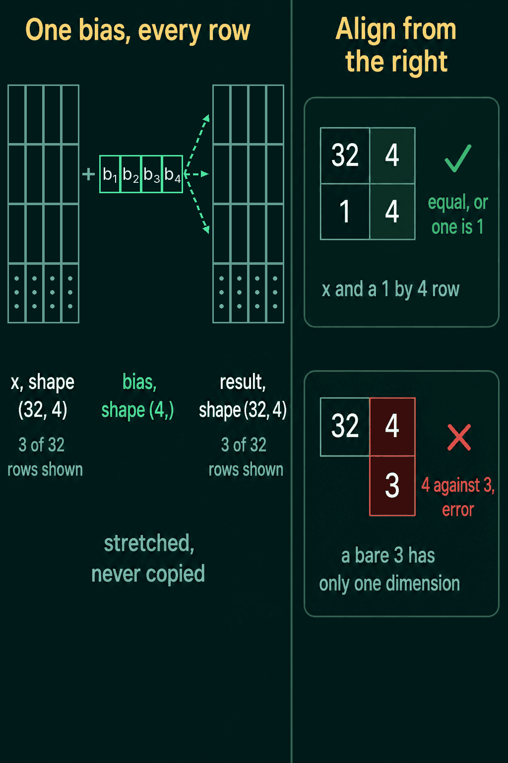
Left: x with shape (32, 4) plus bias with shape (4,) gives a result of shape (32, 4), with the bias row b1 to b4 stretched down every row, never copied. Right: aligning shapes from the right, (32, 4) against (1, 4) works because each pair is equal or one is 1, while (32, 4) against (3) fails because 4 against 3 is an error

The same thing happens inside nn.Linear. Its bias has shape (out_features,), and the layer computes the input times the transposed weight plus that bias, which broadcasts it across the whole batch:

1import torch
2import torch.nn as nn
3 
4torch.manual_seed(0)
5layer = nn.Linear(4, 6)
6x = torch.randn(32, 4)
7 
8print(layer.bias.shape)
9manual = x @ layer.weight.T + layer.bias   # (32, 6) + (6,)
10print(manual.shape, torch.allclose(layer(x), manual))

1torch.Size([6])
2torch.Size([32, 6]) True

Both sides can stretch

The rule applies to each axis separately, so both tensors can stretch at once. A tensor of shape $(3, 1)$ plus one of shape $(1, 4)$ gives $(3, 4)$: the first stretches across columns, the second across rows, and the result holds every pairwise combination of the 3 values and the 4 values, with no loop.

Applied to one vector against itself, v.unsqueeze(1) - v.unsqueeze(0) builds a table of all pairwise differences. unsqueeze(1) turns shape $(3,)$ into a column $(3, 1)$, and unsqueeze(0) turns it into a row $(1, 3)$.

1import torch
2 
3x = torch.ones(32, 4)
4bias = torch.tensor([1.0, 2.0, 3.0, 4.0])
5out = x + bias
6print(out.shape)
7print(out[0], out[31])
8 
9a = torch.arange(3).reshape(3, 1)        # (3, 1)
10b = torch.arange(4).reshape(1, 4) * 10   # (1, 4)
11print(a + b)
12 
13v = torch.tensor([1.0, 4.0, 9.0])
14print(v.unsqueeze(1) - v.unsqueeze(0))   # every pairwise difference

1torch.Size([32, 4])
2tensor([2., 3., 4., 5.]) tensor([2., 3., 4., 5.])
3tensor([[ 0, 10, 20, 30],
4        [ 1, 11, 21, 31],
5        [ 2, 12, 22, 32]])
6tensor([[ 0., -3., -8.],
7        [ 3.,  0., -5.],
8        [ 8.,  5.,  0.]])

The first row and the last row of out got the same bias. In the grid, entry $(i, j)$ is $a_i + b_j$, and in the difference table entry $(i, j)$ is $v_i - v_j$, so $9 - 1 = 8$ sits in row 2, column 0.

Choosing which way a vector stretches

Whether a vector stretches down the rows or across the columns depends on where its size-1 axis is, and you choose that. To scale each of the 32 rows of a $(32, 4)$ batch by its own number, a tensor of shape $(32,)$ does not work: alignment starts from the right, so 32 is compared with 4, and the shapes do not match. scale.unsqueeze(1) makes it $(32, 1)$, which stretches across the 4 features and multiplies each row by one number. A tensor of shape $(4,)$ is the other case: one number per feature, applied the same way down all 32 rows.

When shapes cannot broadcast, PyTorch raises an error instead of guessing. Shapes $(32, 4)$ and $(3,)$ fail, because 4 and 3 are both bigger than 1 and are not equal:

1import torch
2 
3x = torch.ones(32, 4)
4scale = torch.arange(32.0)               # one number per row
5 
6try:
7    x * scale
8except RuntimeError as e:
9    print(e)
10 
11out = x * scale.unsqueeze(1)             # (32, 1) stretches across the 4 features
12print(out.shape)
13print(out[2])
14 
15try:
16    x + torch.ones(3)
17except RuntimeError as e:
18    print(e)

1The size of tensor a (4) must match the size of tensor b (32) at non-singleton dimension 1
2torch.Size([32, 4])
3tensor([2., 2., 2., 2.])
4The size of tensor a (4) must match the size of tensor b (3) at non-singleton dimension 1

A "non-singleton dimension" in the message is an axis whose size is not 1, so the error names the axis where the two sizes clashed. When it appears, print both shapes, align them from the right, and add the missing size-1 axis with unsqueeze where the stretch should happen.

Common mistakes

A per-row value with shape $(n,)$. It lines up with the last axis, the features, not the rows. Give it shape $(n, 1)$.
A square batch hides the bug. If the batch size equals the number of features, say $(4, 4)$, a per-row vector of shape $(4,)$ broadcasts without an error and gets applied per column instead. Testing with a batch size that differs from every other axis size catches this.
An accidental grid. Subtracting a $(32,)$ prediction tensor from a $(32, 1)$ target tensor broadcasts to $(32, 32)$ instead of failing, and a loss averaged over that grid compares every prediction with every target. Check that both have the same shape before the subtraction.
Copying data to match shapes by hand. Repeating a bias 32 times before adding it gives the same result as broadcasting and uses more memory, because the stretched axis reuses the same numbers.

The elementwise product that broadcasting extends is in Hadamard product vs matrix multiplication. Reading shapes and adding axes with unsqueeze is in what is a tensor?. NumPy arrays follow the same broadcasting rule.

QuiddityML teaches broadcasting as a concept in the linear algebra part of the Math track, and the exercises include predicting what a broadcast does before running it, tracing the result shape of several broadcasts against a $(32, 4)$ batch, and writing an add_bias function from scratch.