By Sagi Shaier · 8 October 2026 · 5 min read

Hadamard product vs matrix multiplication: * vs @ in PyTorch

The Hadamard product multiplies two matrices position by position, which is what * does in PyTorch, while matrix multiplication combines rows with columns, which is what @ does. This post compares the two on the same numbers, explains the shape rules for each, and shows where the Hadamard product is used in models.

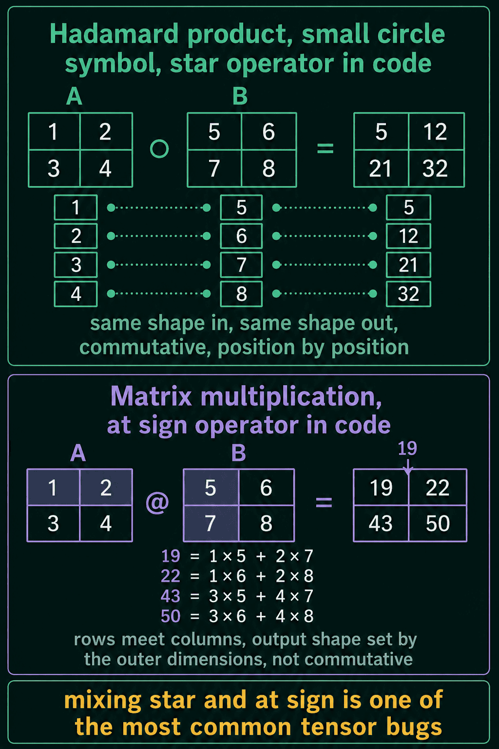
The Hadamard product, also called the elementwise product, multiplies two matrices of the same shape position by position: the top-left entry of one times the top-left entry of the other, and so on for every position. In PyTorch it is the * operator. It is easy to confuse with matrix multiplication, which PyTorch writes as @, and on two square matrices both run without an error while giving completely different numbers.

What the Hadamard product does

A matrix is a grid of numbers with a shape written rows $\times$ columns. Given two matrices $A$ and $B$ with the same shape, the Hadamard product $A \circ B$ is a matrix of that same shape where each entry is the product of the two entries in the same position. The small circle $\circ$ is the usual symbol for it:

$$(A \circ B){ij} = A{ij} \cdot B_{ij}$$

Here $A_{ij}$ is the entry of $A$ in row $i$ and column $j$. Nothing is combined across positions: entry $(1, 2)$ of the result depends only on entry $(1, 2)$ of each input.

With $A = \begin{bmatrix} 1 & 2 \ 3 & 4 \end{bmatrix}$ and $B = \begin{bmatrix} 5 & 6 \ 7 & 8 \end{bmatrix}$:

$$A \circ B = \begin{bmatrix} 5 & 12 \ 21 & 32 \end{bmatrix}$$

What matrix multiplication does instead

Matrix multiplication $AB$ builds each entry from a whole row of $A$ and a whole column of $B$. Entry $(i, j)$ of $AB$ is row $i$ of $A$ times column $j$ of $B$, entry by entry, with the products added up. For the top-left entry of the same two matrices, that is $1 \cdot 5 + 2 \cdot 7 = 19$, and the full result is

$$AB = \begin{bmatrix} 19 & 22 \ 43 & 50 \end{bmatrix}$$

The same two inputs give $\begin{bmatrix} 5 & 12 \ 21 & 32 \end{bmatrix}$ one way and $\begin{bmatrix} 19 & 22 \ 43 & 50 \end{bmatrix}$ the other. Both results look like reasonable numbers, which is why using one operator in place of the other produces output that looks plausible and is wrong.

Top: A times B with the Hadamard product, each of the four entries 1, 2, 3, 4 paired with 5, 6, 7, 8 in the same position to give 5, 12, 21, 32. Bottom: A at-sign B with matrix multiplication giving 19, 22, 43, 50, with 19 equals 1 times 5 plus 2 times 7 and the other three entries worked out the same way

The shape rules and the order rule

The two operations have different rules about shapes and order:

	Hadamard product	Matrix multiplication
PyTorch operator	`*`	`@`
Input shapes	same shape	inner dimensions match
Output shape	same as inputs	outer dimensions
Order changes the result	no	yes

The Hadamard product needs both matrices to have the same shape, since every entry needs a partner in the same position, and the result keeps that shape. Matrix multiplication of an $m \times p$ matrix by a $p \times n$ matrix needs the two $p$ values to match and gives an $m \times n$ result.

The Hadamard product is commutative, meaning $A \circ B = B \circ A$, because multiplying two single numbers gives the same answer in either order. Matrix multiplication is not commutative: $AB$ and $BA$ are usually different, and one of them may not even exist.

* and @ in PyTorch

1import torch
2 
3A = torch.tensor([[1., 2.],
4                  [3., 4.]])
5B = torch.tensor([[5., 6.],
6                  [7., 8.]])
7 
8print(A * B)                     # Hadamard product: position by position
9print(A @ B)                     # matrix multiplication: rows meet columns
10print(torch.equal(A * B, B * A), torch.equal(A @ B, B @ A))
11 
12# shapes: @ needs matching inner dimensions, * needs matching shapes
13X = torch.ones(2, 3)
14Y = torch.ones(3, 2)
15print((X @ Y).shape)
16try:
17    X * Y
18except RuntimeError as e:
19    print("RuntimeError:", str(e).split("\n")[0])
20 
21# gating: values between 0 and 1 decide how much of each entry gets through
22h = torch.tensor([2.0, -1.0, 4.0, 3.0])
23gate = torch.tensor([1.0, 0.5, 0.0, 0.25])
24print(h * gate)
25 
26# masking: the same trick with only 0s and 1s
27scores = torch.tensor([0.9, 0.4, 0.7, 0.2])
28mask = torch.tensor([1.0, 1.0, 0.0, 0.0])   # last two positions are padding
29print(scores * mask)

1tensor([[ 5., 12.],
2        [21., 32.]])
3tensor([[19., 22.],
4        [43., 50.]])
5True False
6torch.Size([2, 2])
7RuntimeError: The size of tensor a (3) must match the size of tensor b (2) at non-singleton dimension 1
8tensor([ 2.0000, -0.5000,  0.0000,  0.7500])
9tensor([0.9000, 0.4000, 0.0000, 0.0000])

A $2 \times 3$ matrix and a $3 \times 2$ matrix can be matrix-multiplied into a $2 \times 2$ result, and the same pair fails with * because the shapes differ. When a result has numbers that look reasonable but a model trains badly, checking every * and @ against the operation the math calls for is a quick first step.

Where the Hadamard product shows up

Gating multiplies a vector position by position with a second vector of values between 0 and 1. Each gate value decides how much of the matching entry gets through: 1 keeps all of it, 0.5 keeps half, and 0 blocks it. In the code above, the gate $(1, 0.5, 0, 0.25)$ turns $(2, -1, 4, 3)$ into $(2, -0.5, 0, 0.75)$.

Masking is the same operation with a vector of only 0s and 1s. Multiplying by the mask keeps the positions marked 1 and sets the positions marked 0 to zero, which is a common way to make a model ignore padding added to the end of shorter inputs. Both patterns appear in many model architectures.

Common mistakes

Writing * where the math says matrix multiplication. On square matrices this runs and returns wrong numbers with no error.
Writing @ where the math says $\circ$. A gate or mask applied with @ mixes positions together, so the output no longer lines up with the input.
Expecting * to check shapes strictly. PyTorch's * also accepts some different shapes by repeating the smaller tensor along missing dimensions, a rule called broadcasting, so a $(2, 3)$ tensor times a $(3,)$ tensor runs and gives a $(2, 3)$ result.
Swapping the order of @. B * A gives the same result as A * B, while B @ A usually differs from A @ B.

Matrix multiplication itself, with the row-times-column rule, the transformation view and outer products, is covered in matrix multiplication explained. Vectors and matrices, including shapes and indexing, are in vectors and matrices for machine learning.

QuiddityML teaches the Hadamard product as its own concept in the linear algebra part of the Math track, and the exercises on it include picking the code that computes $A \circ B$, spotting the buggy line in an apply_gate function, and writing apply_gate from scratch.