By Sagi Shaier · 10 October 2026 · 6 min read

SVD explained: singular value decomposition and low-rank approximation

What the three factors of an SVD do to a vector, how to read a matrix's rank off its singular values, and how keeping only the largest few gives the closest possible low-rank copy of the matrix, with PyTorch code for each.

The singular value decomposition (SVD) splits any matrix into three simpler matrices: one that rotates, one that stretches along the axes, and one that rotates again. It works for every matrix, square or rectangular, and it is behind PCA, recommender systems, and compressing large embedding or weight matrices down to their strongest directions.

Why eigendecomposition is not enough

An eigenvector of a square matrix $A$ is a direction that $A$ only stretches, without turning it, and the stretch factor is its eigenvalue. Eigendecomposition rewrites a matrix using its eigenvectors and eigenvalues, and it has two limits. It only applies to square matrices, and even some square matrices do not have enough eigenvectors to be decomposed this way.

Many matrices in machine learning are rectangular: a dataset with 10,000 rows and 50 features, or a weight matrix that maps 768 numbers to 3,072. SVD removes both limits, because every matrix has one.

The decomposition

For a matrix $A$ with $m$ rows and $n$ columns, the SVD is

$$A = U\Sigma V^\top$$

where:

$U$ is an $m \times m$ orthogonal matrix. Its columns all have length 1 and are at right angles to each other, so multiplying by it rotates or reflects a vector without changing its length.
$V$ is an $n \times n$ orthogonal matrix, and $V^\top$ is its transpose.
$\Sigma$ (capital sigma) is an $m \times n$ diagonal matrix, with zeros everywhere off the main diagonal. The numbers on its diagonal, written $\sigma_1, \sigma_2, \ldots$, are the singular values. They are never negative and are listed from largest to smallest.

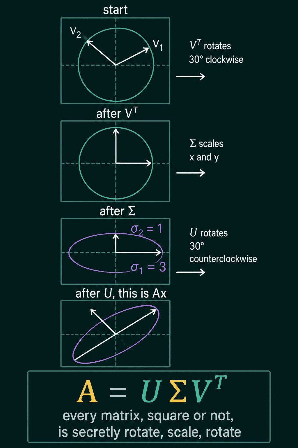
Read right to left, $A\mathbf{x} = U\Sigma V^\top\mathbf{x}$ does three things to a vector $\mathbf{x}$: $V^\top$ rotates or reflects it, $\Sigma$ stretches each axis by its singular value (and changes the number of dimensions when $m \neq n$), and $U$ rotates or reflects the result into place. Every matrix comes apart into rotate, scale, rotate.

A 2 by 2 example of SVD drawn in four panels: a circle with two directions v1 and v2, then V transpose rotates it 30 degrees clockwise so v1 and v2 line up with the axes, then Sigma stretches x by sigma 1 = 3 and y by sigma 2 = 1 into an ellipse, then U rotates the ellipse 30 degrees counterclockwise, giving Ax

The thin SVD

The full shapes carry padding. When $m > n$, $\Sigma$ has only $n$ diagonal entries, and the last $m - n$ columns of $U$ only ever multiply rows of zeros in $\Sigma$. The thin (or reduced, or economy) SVD drops them. With $k = \min(m, n)$, torch.linalg.svd(A, full_matrices=False) returns $U$ of shape $m \times k$, the singular values as a flat vector of length $k$, and $V^\top$ of shape $k \times n$. The product is the same matrix, and this is the version used for compression.

Rank from singular values

The rank of a matrix is the number of independent directions its columns span. A matrix with three columns where the third is the sum of the first two has rank 2, because the third column adds no new direction.

The SVD makes rank a counting question: the rank of $A$ is the number of nonzero singular values. Floating-point arithmetic rarely produces an exact zero, so code counts the singular values above a small threshold instead. A value like $10^{-16}$ next to a largest value of 4.6 is zero in every practical sense.

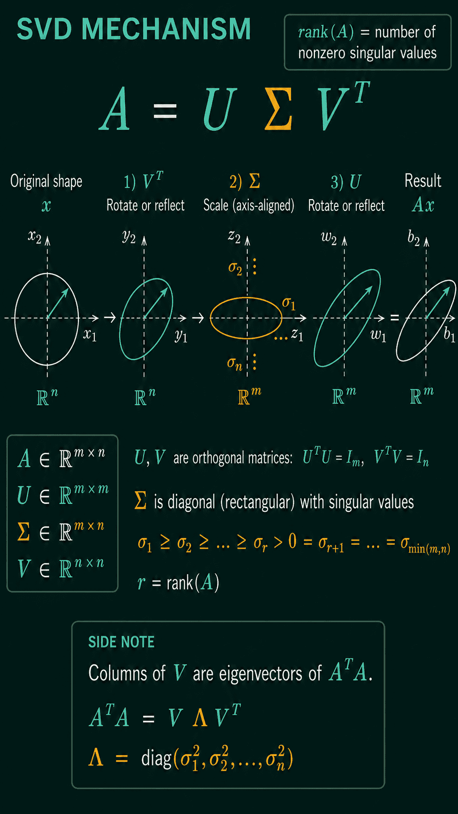
SVD mechanism: A = U Sigma V transpose drawn as rotate or reflect, scale along the axes, rotate or reflect, with U in R m by m, Sigma m by n, V n by n, singular values sorted sigma 1 >= sigma 2 >= ... >= sigma r > 0 followed by zeros, r = rank of A, and a side note that the columns of V are eigenvectors of A transpose A with eigenvalues sigma squared

The image also shows where SVD comes from. The columns of $V$ are the eigenvectors of $A^\top A$, the columns of $U$ are the eigenvectors of $AA^\top$, and each singular value is the square root of the matching eigenvalue. $A^\top A$ is square and symmetric even when $A$ is neither, and a symmetric matrix always has a full set of eigenvectors, which is how SVD avoids the limits of eigendecomposition.

1import torch
2 
3torch.manual_seed(0)
4# A 5x3 matrix whose third column is the sum of the first two, so its rank is 2
5B = torch.randn(5, 2, dtype=torch.float64)
6A = torch.cat([B, B.sum(dim=1, keepdim=True)], dim=1)
7 
8U, S, Vt = torch.linalg.svd(A, full_matrices=False)
9print(U.shape, S.shape, Vt.shape)
10print(S)
11 
12A_rebuilt = U @ torch.diag(S) @ Vt
13print(torch.allclose(A, A_rebuilt))
14 
15rank = (S > 1e-10 * S[0]).sum().item()
16print(rank, torch.linalg.matrix_rank(A).item())

1torch.Size([5, 3]) torch.Size([3]) torch.Size([3, 3])
2tensor([4.6111e+00, 2.0156e+00, 1.7967e-16], dtype=torch.float64)
3True
42 2

The thin SVD of the $5 \times 3$ matrix has $U$ of shape $5 \times 3$, three singular values, and $V^\top$ of shape $3 \times 3$. torch.diag(S) turns the vector of singular values back into a diagonal matrix, and the product rebuilds $A$. The third singular value is about $10^{-16}$, so the count above the threshold is 2, the same answer torch.linalg.matrix_rank gives.

Low-rank approximation

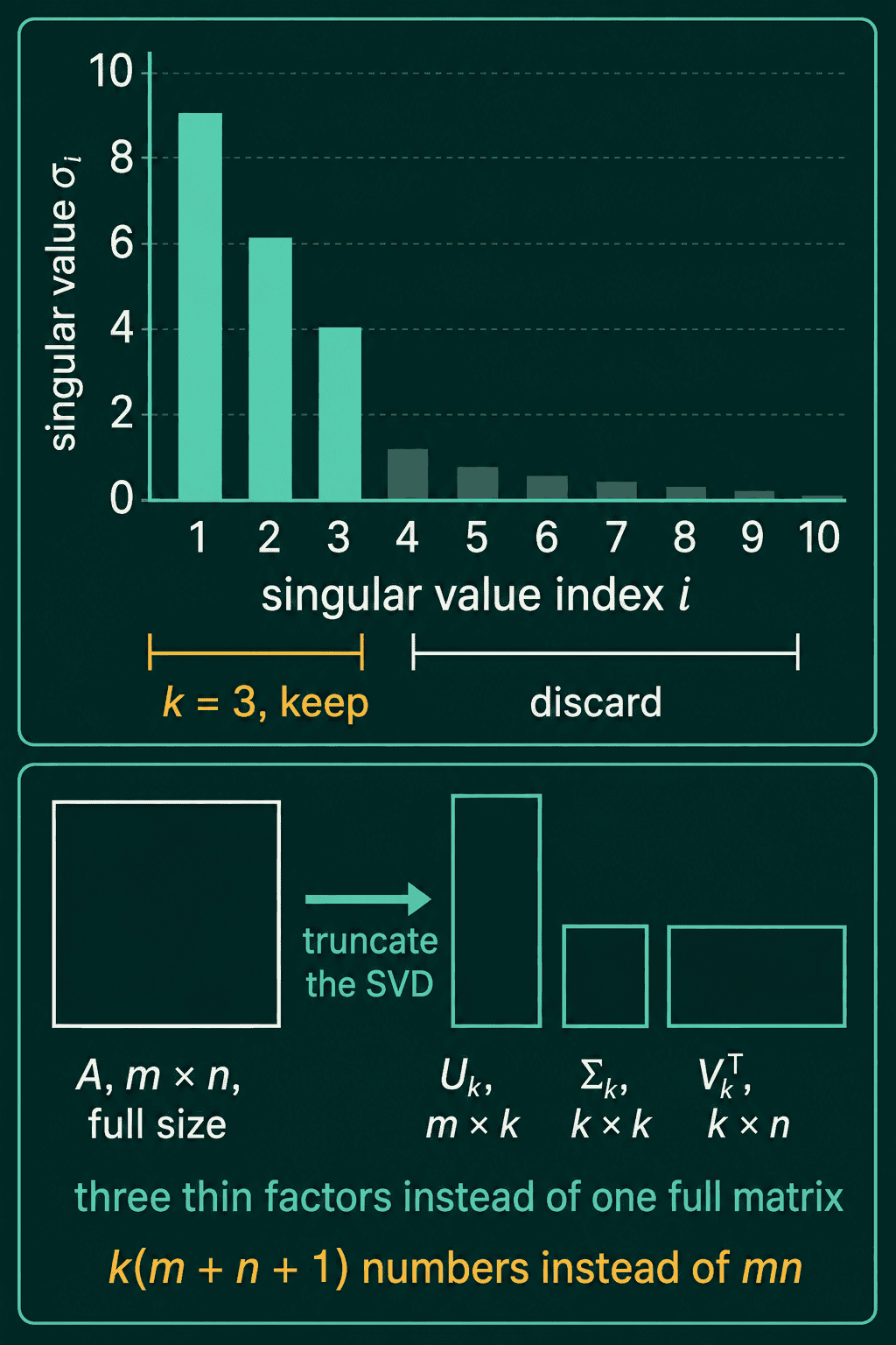
Because the singular values are sorted, the first few carry the strongest structure in $A$, and the last few often carry very little, sometimes not much more than noise. Low-rank approximation keeps the top $k$ singular values, along with the first $k$ columns of $U$ and the first $k$ rows of $V^\top$, and drops the rest:

$$A_k = U_k \Sigma_k V_k^\top$$

$U_k$ is $m \times k$, $\Sigma_k$ is the $k \times k$ diagonal of the largest singular values, and $V_k^\top$ is $k \times n$. The result $A_k$ has the same shape as $A$ and rank $k$.

A bar chart of 10 singular values: the first three (about 9, 6 and 4) are kept with k = 3, and the remaining seven, all below about 1.2, are discarded. Below it, the full m by n matrix A becomes three thin factors U k (m by k), Sigma k (k by k) and V k transpose (k by n)

This is more than a convenient shortcut. Measure the error with the Frobenius norm, the square root of the sum of every squared entry of $A - B$, written $\|A - B\|_F$. Among all matrices $B$ of rank $k$, none gets $\|A - B\|_F$ smaller than $A_k$ does, and the error left over is set by the singular values that were dropped:

$$\|A - A_k\|_F = \sqrt{\sigma_{k+1}^2 + \cdots + \sigma_r^2}$$

where $r$ is the rank of $A$. Once $k$ reaches $r$, nothing is dropped and the error is zero.

How much it saves

The rank-$k$ version stores $k$ columns of $U$, $k$ rows of $V^\top$, and $k$ singular values. For a $1000 \times 1000$ matrix that is 1,000,000 numbers in full, and a rank-10 approximation stores

$$10 \times 1000 + 10 \times 1000 + 10 = 20{,}010$$

numbers, about 2% of the original. When the matrix is close to rank 10, the compressed copy loses little.

1import torch
2 
3torch.manual_seed(0)
4# Rank-3 structure plus a little noise
5A = torch.randn(100, 3) @ torch.randn(3, 80) + 0.05 * torch.randn(100, 80)
6 
7U, S, Vt = torch.linalg.svd(A, full_matrices=False)
8print(S[:6].round(decimals=2))
9 
10k = 3
11A_k = U[:, :k] @ torch.diag(S[:k]) @ Vt[:k, :]
12 
13error = torch.linalg.norm(A - A_k)            # Frobenius norm
14predicted = torch.sqrt((S[k:] ** 2).sum())    # from the discarded singular values
15print(round(error.item(), 4), round(predicted.item(), 4))
16 
17full = A.numel()
18stored = k * A.shape[0] + k * A.shape[1] + k
19print(full, stored)
20print(round((error / torch.linalg.norm(A)).item(), 4))

1tensor([106.1400,  92.7100,  79.1000,   0.9100,   0.8900,   0.8700])
24.319 4.319
38000 543
40.0267

The matrix is built from a rank-3 product plus small random noise, and the singular values show it: three large ones (106, 93, 79) and then a drop to below 1. Keeping $k = 3$ gives an error of 4.319, exactly the square root of the sum of the dropped singular values squared. The rank-3 copy stores 543 numbers instead of 8,000, and its error is about 2.7% of the size of $A$. If the error comes out larger than expected, print the singular values first: a slow, gradual decay means the matrix has no small $k$ that captures most of it.

When to use it, and common mistakes

SVD is a common choice for computing rank, for compressing a matrix that is close to low rank, and for PCA, where the top singular directions of a centered data matrix are the directions of greatest variance.

Computing the full SVD when the thin one is enough. For a tall matrix, full_matrices=True builds a large $U$ whose extra columns multiply zeros. Pass full_matrices=False.
Testing singular values against exact zero. Rounding leaves values like $10^{-16}$, so compare against a threshold scaled to the largest singular value.
Slicing the wrong axis of Vt. torch.linalg.svd returns $V^\top$, so the top $k$ directions are its first $k$ rows, Vt[:k, :], and the first $k$ columns of $U$, U[:, :k].
Expecting compression on a matrix that is not close to low rank. If the singular values decay slowly, a small $k$ throws away a lot.

Eigenvalues and eigenvectors, which SVD generalizes to any matrix, are in eigenvalues and eigenvectors explained. Rank and the column space are in rank, column space and null space explained. The condition number of a general matrix is the largest singular value divided by the smallest, covered in the condition number explained. Low-rank adaptation methods for large pretrained models, LoRA among them, use the same idea of a weight change built from two thin matrices, though they learn those factors by training instead of truncating an SVD.

QuiddityML teaches SVD and low-rank approximation as two concepts in the linear algebra part of the Math track, and the exercises include tracing the shapes of the thin SVD factors, spotting the bug in a low_rank_approx function, and writing it from scratch.