2 October 2026 · 7 min read

The curse of dimensionality explained

The curse of dimensionality is what happens to a dataset when you add input features without adding examples. This post shows why the same data covers less of the input space with each new feature, why distances between examples stop being useful, and what to do about it.

The curse of dimensionality is the name for what happens to a fixed dataset as the number of input features grows: the examples cover a smaller and smaller share of the possible inputs. Adding a feature looks like adding one more column to a table, and it can still make a model worse, because the model now has to make predictions in regions where it has seen few or no examples.

What a dimension is

A feature is one measured property of an example, such as the size of a house. Each feature is one dimension of the input. A dataset with three features per example has three-dimensional inputs, and the set of every possible combination of feature values is called the input space. A model learns from the parts of the input space where it has training examples.

The same 100 examples in a larger space

Take a house-price dataset with 100 houses and one feature, house size. To measure coverage, split the size axis into 10 buckets: 0 to 500 sq ft, 500 to 1,000 sq ft, and so on. If the houses are spread evenly, each bucket holds about 10 of them. A new 1,600 sq ft house lands in a bucket with around 10 training houses of similar size.

Add a second feature, distance from downtown, and split it into 10 buckets too. Each house now falls into a cell with two coordinates, one size bucket and one distance bucket. Ten size buckets times ten distance buckets is $10^2 = 100$ cells, so the same 100 houses average one per cell.

Add house age as a third feature with 10 buckets. There are now $10^3 = 1{,}000$ cells and still 100 houses, so at most one cell in ten contains a house and the rest are empty.

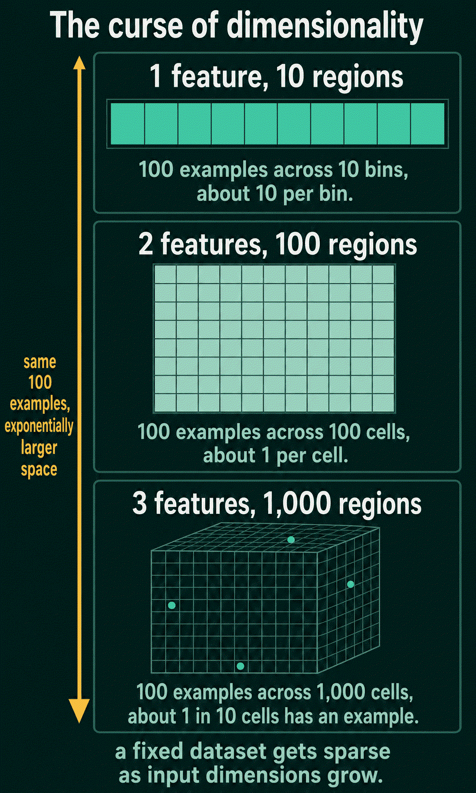
The same 100 examples spread over 10 regions with one feature, 100 cells with two features, and 1,000 cells with three features, where about one cell in ten has an example.

With $k$ features and 10 buckets each, the number of cells is $10^k$. The number of cells is multiplied by 10 with each feature, while the dataset stays the same size. At 10 features there are 10 billion cells, and a house dataset with thousands of rows fills a tiny fraction of them. This growth is the curse of dimensionality: as the number of input dimensions grows, a fixed dataset becomes sparse in the input space.

What sparse data does to a model

A model predicts well for a new input when it has seen training examples that resemble it. In a sparse dataset, a new input has few examples nearby, so the prediction rests on examples that differ from it in several features at once.

Sparsity also gives the model more room to fit accidents. With many features and few examples, some feature will line up with the labels in the training set by chance. A model with enough freedom picks up that chance pattern, its training loss drops, and its loss on new data does not follow. That is overfitting, which means fitting the training set more closely than the real pattern justifies.

Why distance gets weaker

Many methods decide which training examples are relevant to a new input by measuring distance. The usual measure is Euclidean distance: subtract the two examples feature by feature, square each difference, add the squares, and take the square root.

Take a new input, called the query, and one training example. With a single feature $x$, the query sits at 0 and the example at 1, so the distance is 1. Add a second feature $y$ on which the two differ by 4. The query is at $(0, 0)$, the example is at $(1, 4)$, and the distance is $\sqrt{1^2 + 4^2} = 4.12$. Add a third feature $z$ on which they differ by 7, and the distance is $\sqrt{1^2 + 4^2 + 7^2} = 8.12$. The two points are still only 1 apart on $x$, but each added feature is another way for them to differ, and every difference adds to the total.

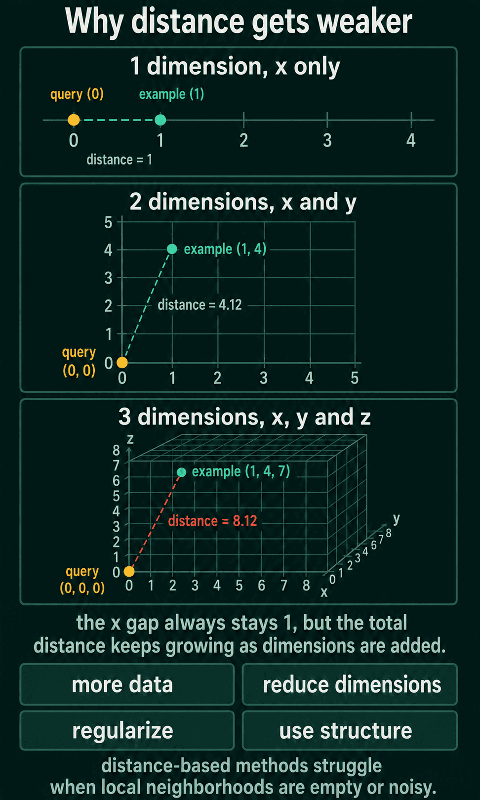
A query and an example that are 1 apart on one axis, 4.12 apart once a second axis is added, and 8.12 apart with a third, followed by four responses: more data, reduce dimensions, regularize, use structure.

The larger problem is what happens to all the distances together. When there are many features, every training example ends up roughly the same distance from the query, so the nearest example is barely nearer than the farthest one. A method that relies on "the closest examples" is then choosing among examples that are all about equally far away.

Code

The snippet draws 1,000 random examples and one query, with each feature uniform between 0 and 1, and compares the query's distance to its nearest and farthest example as the number of dimensions grows.

1import torch
2 
3torch.manual_seed(0)
4n = 1000                                            # same number of examples every time
5 
6for dims in (1, 2, 10, 100, 1000):
7    data = torch.rand(n, dims)                      # each feature uniform in [0, 1]
8    query = torch.rand(1, dims)                     # one new point
9    dist = torch.cdist(query, data).squeeze(0)      # distance to every example
10    nearest, farthest = dist.min().item(), dist.max().item()
11    print(f"dims={dims:4d}  nearest={nearest:6.3f}  farthest={farthest:6.3f}  nearest/farthest={nearest / farthest:.2f}")

1dims=   1  nearest= 0.000  farthest= 0.542  nearest/farthest=0.00
2dims=   2  nearest= 0.008  farthest= 0.887  nearest/farthest=0.01
3dims=  10  nearest= 0.540  farthest= 2.060  nearest/farthest=0.26
4dims= 100  nearest= 3.286  farthest= 4.749  nearest/farthest=0.69
5dims=1000  nearest=12.266  farthest=13.659  nearest/farthest=0.90

With one or two features the nearest example is almost at the same position as the query. At 100 features the nearest example is 69% as far away as the farthest, and at 1,000 features it is 90% as far. The 1,000 examples did not change, only the number of dimensions they are spread over.

Which methods are affected most

The effect is most direct in methods that use distance explicitly. K-nearest neighbors predicts the label of a new input from the labels of the $k$ closest training examples, so it depends on "closest" meaning something. Clustering methods group examples by distance, and kernel methods weight training examples by how close they are to the input.

Neural networks do not predict by voting over nearby examples, but they still learn from a finite set of examples spread over the input space, so sparse coverage raises their risk of overfitting too.

What to do about it

High-dimensional problems usually need one of four responses.

More data, so more regions of the input space contain examples.
Dimensionality reduction, which replaces the original features with a smaller set that keeps most of the information. Principal component analysis is a common method: it finds the directions along which the data varies most and keeps only those.
Regularization, the set of techniques that limit how closely a model can fit its training set, such as weight decay and dropout, so the model has less freedom to fit chance patterns.
Structure in the model, so the architecture builds in assumptions about the data. A convolutional network assumes that nearby pixels are related and that a pattern means the same thing wherever it appears in the image, which lets it learn from far fewer images than a model that treats each pixel as an unrelated feature.

Why high-dimensional learning still works

A 224 by 224 color image has 150,528 input values, and models learn from images anyway. The bucket argument assumes the examples could land anywhere in the input space, and real data does not behave that way. Neighboring pixels are strongly correlated, so real images occupy a small part of the space of all possible pixel grids. The number of directions in which the data really varies is much lower than the number of raw features, and that lower number is the one that sets how much data is needed.

So the curse does not say high-dimensional learning fails. It says that each extra input dimension asks more of the dataset, the model, or the assumptions built into the model.

Common mistakes

Adding features because they might help. A weak or noisy feature adds a dimension to cover and a new chance to fit an accident, and it can lower validation accuracy even though it carries a little signal.

Running k-nearest neighbors or clustering on raw high-dimensional inputs. Reducing the dimensions first, or measuring distance in a learned representation, usually makes the nearest examples more relevant.

Judging a dataset by its number of rows alone. A thousand examples is a lot for 3 features and very little for 300, so the count has to be read against the number of features.

Checking only training accuracy after adding features. More features usually make the training set easier to fit, and the validation set is where the cost shows up.

Overfitting is the failure that sparse coverage leads to, and the curse of dimensionality is one reason it gets more likely as features are added. The question of how much data a model needs is the same problem seen from the data side, since more dimensions and more parameters both raise the requirement. Feature selection, which keeps only the features that help validation performance, is a simpler relative of dimensionality reduction.

QuiddityML teaches the curse of dimensionality as its own concept in the ML Foundation track, and the exercises ask what goes wrong when 30 weak features are added to 1,000 examples and why a k-nearest-neighbors classifier gets worse after 100 noisy features are added.