2 October 2026 · 7 min read

Double descent explained

Double descent is what happens when a model keeps growing after it can fit its training data exactly. Its error on new data rises to a peak and then falls a second time. This post explains where the peak sits, why very large models can do better than mid-sized ones, and how to reproduce the curve in a few lines of PyTorch.

Double descent is a pattern in how a model's error on new data changes as the model gets larger: the error falls, rises to a peak, and then falls a second time. The standard advice says a model that is too large for its dataset overfits, so the fix is to shrink it. Double descent shows that growing the model well past that point can also work, which is part of why networks with far more parameters than training examples do well in practice.

The classic picture: a U-shaped curve

Training error is a model's error on the examples it was trained on. Test error is its error on examples it never saw, and it is the number that says whether the model works. Model complexity, also called capacity, is how many different functions the model can represent, and for a neural network it grows with the number of parameters.

In the classic picture, test error plotted against model complexity traces a U. A very small model cannot represent the pattern in the data, so both errors are high. As the model grows it captures more of the pattern and test error falls. Past a certain size the model has enough freedom to fit the random noise in the training labels as well, which is called overfitting, and test error rises again. The bottom of the U is the model size that balances the two, and choosing it is the usual goal.

What happens past the top of the U

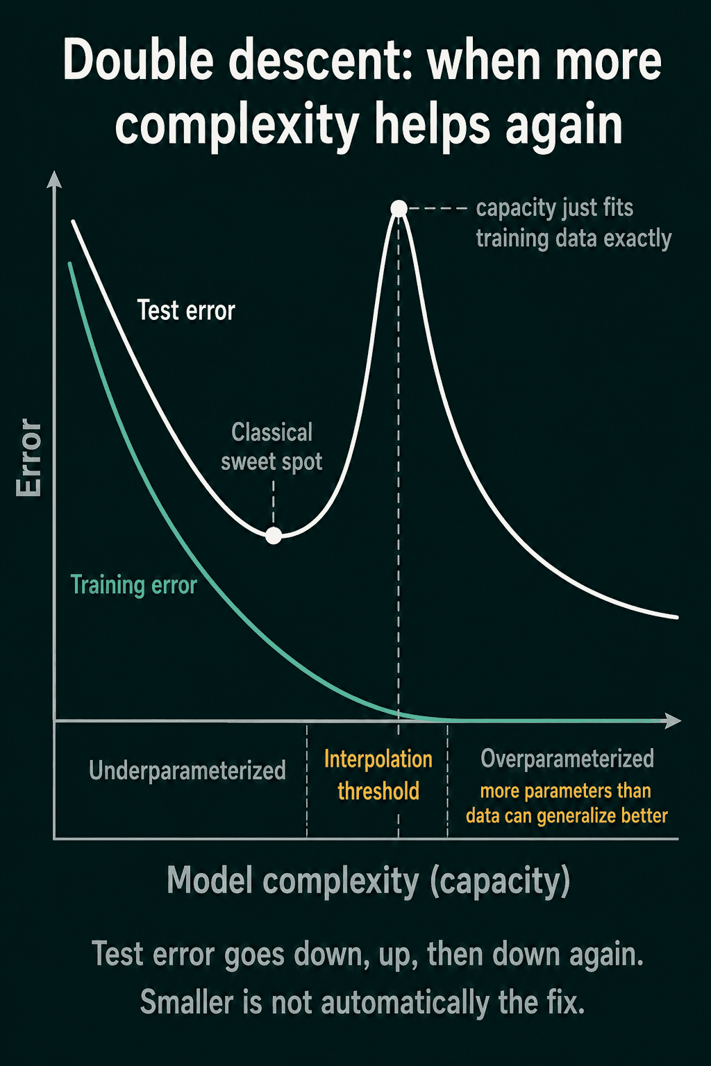
Keep growing the model and it reaches a size where it fits every training example exactly, so its training error is zero. Fitting the training data exactly is called interpolating it, and the smallest model size that can do it is the interpolation threshold. Models below the threshold are called underparameterized, and models above it are called overparameterized.

The U-curve predicts that test error keeps climbing past this point. What is observed in many experiments is different. Test error peaks near the interpolation threshold, and then falls again as the model grows further. With enough extra capacity it can drop below the bottom of the original U. Down, up, then down a second time is the shape that gives double descent its name.

Why the peak sits at the threshold

There is no settled explanation, and the common one goes like this. Right at the threshold, the model has barely enough capacity to pass through every training point. Very few settings of its parameters achieve that, sometimes exactly one, and the model has no freedom left over to choose a sensible one. The training labels contain noise, so the single function that fits all of them tends to swing sharply between points to hit each noisy label. Those swings are large errors on any new input.

Well past the threshold the situation changes. A model with far more capacity than it needs can fit the training set exactly in many different ways. The training procedure does not pick among them at random. Gradient descent started from small weights tends to end at a fit with small weights, and fits with small weights are usually smoother functions. A smoother function that still passes through the training points makes smaller errors between them.

So the same zero training error can come from a fit forced through every point at the threshold or from a smooth fit far beyond it, and the test error of the two is very different.

Where to look for the peak

As a rule of thumb, the interpolation threshold sits roughly where the number of parameters matches the number of training examples. That is the model size with enough capacity to fit every point and none to spare. The rule is approximate, because the capacity a model uses in practice is not the same as its raw parameter count, but it says where in a sweep of model sizes the peak is likely to appear.

Regularization changes the curve. Regularization is the set of techniques that hold a model back from fitting its training set too closely. Weight decay is one of them: it adds a penalty for large weights, which pushes the model toward smoother functions. Early stopping is another: training is stopped before the model has fully fit the training set. The peak is sharpest for a model that interpolates with nothing constraining how it does so. With weight decay or early stopping, the peak can shrink or disappear.

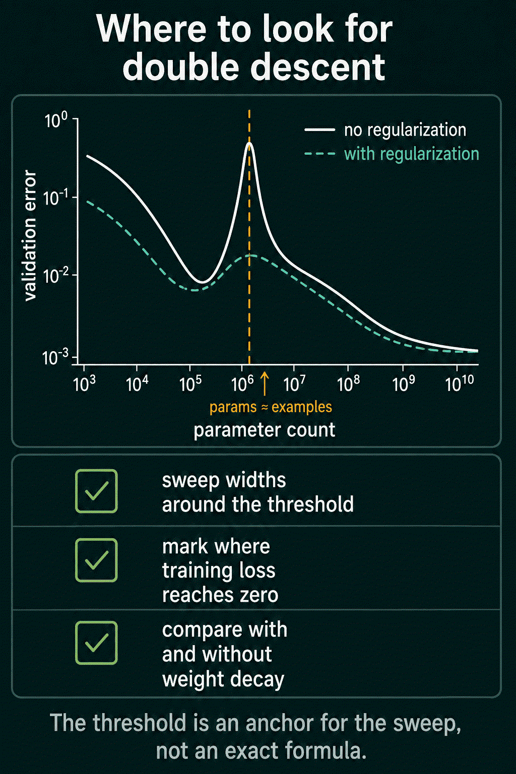
Double descent is therefore not a law that every sweep has to show. Model size, dataset size, the optimizer, and regularization all interact, and the curve to trust is the one measured on the problem at hand.

Code

The snippet reproduces the curve with a small model that needs no training loop. The inputs pass through a fixed random layer followed by a ReLU, and only the last linear layer is fitted, by least squares. The width of the random layer is the number of fitted parameters. There are 100 training examples, so the interpolation threshold is at a width of 100. torch.linalg.pinv returns the least-squares fit, and when many exact fits exist it returns the one with the smallest weights.

1import torch
2 
3torch.manual_seed(0)
4n_train, n_test, d = 100, 2000, 20
5 
6w_true = torch.randn(d, 1)
7def make_data(n):
8    x = torch.randn(n, d)
9    y = x @ w_true + 0.5 * torch.randn(n, 1)       # linear signal plus noise
10    return x, y
11 
12x_train, y_train = make_data(n_train)
13x_test, y_test = make_data(n_test)
14 
15def run(width, ridge=0.0, trials=20):
16    train, test = 0.0, 0.0
17    for _ in range(trials):
18        proj = torch.randn(d, width) / d ** 0.5     # fixed random first layer
19        f_train, f_test = torch.relu(x_train @ proj), torch.relu(x_test @ proj)
20        if ridge:                                   # least squares with a penalty on large weights
21            w = torch.linalg.solve(f_train.T @ f_train + ridge * torch.eye(width), f_train.T @ y_train)
22        else:                                       # plain least squares, smallest weights if many fits exist
23            w = torch.linalg.pinv(f_train) @ y_train
24        train += ((f_train @ w - y_train) ** 2).mean().item() / trials
25        test += ((f_test @ w - y_test) ** 2).mean().item() / trials
26    return train, test
27 
28for width in (10, 25, 50, 90, 100, 110, 200, 500, 2000):
29    train, test = run(width)
30    print(f"width={width:5d}  train={train:8.3f}  test={test:9.3f}")
31 
32print()
33for width in (50, 100, 2000):
34    train, test = run(width, ridge=1.0)
35    print(f"ridge=1.0  width={width:5d}  train={train:8.3f}  test={test:9.3f}")

1width=   10  train=  15.345  test=   20.428
2width=   25  train=   6.836  test=   12.650
3width=   50  train=   2.007  test=    9.266
4width=   90  train=   0.166  test=   19.926
5width=  100  train=   0.000  test=38721.663
6width=  110  train=   0.000  test=   21.361
7width=  200  train=   0.000  test=    2.435
8width=  500  train=   0.000  test=    1.162
9width= 2000  train=   0.000  test=    0.797
10 
11ridge=1.0  width=   50  train=   2.000  test=    6.987
12ridge=1.0  width=  100  train=   0.299  test=    3.981
13ridge=1.0  width= 2000  train=   0.000  test=    0.824

Test error falls to 9.266 at a width of 50, which is the bottom of the classic U. It climbs to 19.926 at a width of 90 and spikes at 100, the width where training error first reaches zero. Past the threshold it falls again, and by a width of 200 it is already at 2.435, well below the bottom of the U. At a width of 2,000, with 20 times more fitted parameters than training examples, it reaches 0.797. The height of the spike at 100 changes a lot from one random seed to the next, but its position does not.

The last three lines repeat the fit with a penalty on large weights, which is what weight decay does. At a width of 100 the test error is 3.981 instead of 38,721, so the peak is gone, and at a width of 2,000 the penalty makes little difference.

Other places the same shape shows up

The curve above is plotted against model size. A similar shape can appear along two other axes. Plotted against training time, test error can fall, rise as the model starts fitting noise, and fall again with much longer training. Plotted against dataset size for a fixed model, adding training examples can briefly make test error worse, when the added examples move the interpolation threshold onto the model's size.

What it means in practice

When a model overfits, a smaller model and a much larger model are both worth trying, and the larger one is often the better choice when there is compute to spare and regularization is in place. This is part of why large networks are trained with weight decay, dropout, or early stopping instead of being cut down to the size the U-curve suggests.

When sweeping model sizes, include sizes well past the point where training error reaches zero. A sweep that stops soon after that point ends at the peak.

Common mistakes

Stopping the sweep at the peak. If the largest model tried sits near the interpolation threshold, the results say that bigger is worse, and the second descent is missed.

Expecting the peak in every experiment. With weight decay, early stopping, data augmentation, or little noise in the labels, the peak is often too small to see, and its absence does not mean anything is wrong.

Using the parameter count as an exact threshold. Parameters roughly equal to examples is a starting point for a sweep, and the place where training error reaches zero is the actual threshold.

Reading double descent as "bigger is always better". The second descent depends on how the model is trained, and a larger model still costs more memory, compute, and time.

Related concepts

The bias-variance tradeoff is the theory behind the U-shaped part of the curve, where a model that is too simple has high bias and a model with too much freedom has high variance. Overfitting is the rise in test error on the right side of the U, and double descent describes what can happen after it. Regularization, which includes weight decay, dropout, and early stopping, is the reason the peak is often flattened in practice.

QuiddityML teaches double descent as its own concept in the ML Foundation track, and the exercises ask where the interpolation threshold sits in a sweep of model widths and what happened when the same sweep with weight decay shows almost no peak.