2 October 2026 · 8 min read

How much data do you need to train a model?

The amount of training data a model needs depends on how large the model is, how accurate it has to be, and how noisy the data is. This post explains that relationship, the formal version from learning theory, and a test that tells you whether more data would help your model.

There is no single number of training examples that is enough. The amount a model needs grows with the size of the model, with how accurate the model has to be, and with how much random noise is in the data. A few dozen examples are usually enough to fit a model with 10 parameters, and nowhere near enough for a model with 10 million. Getting this wrong in one direction wastes time on data collection, and getting it wrong in the other produces a model that scores well on its training data and badly on everything else.

What goes wrong with too little data

The training set is the examples a model updates its parameters on. A held-out set, often called the validation set, is examples the model never trains on, kept aside to measure how the model does on data it has not seen. Real data also contains noise, which is the random part of each label that no input explains, such as measurement error.

A model with many parameters has enough freedom to fit the noise as well as the pattern. With only a few examples, there are many different functions that pass through all of them, and most of those functions are wrong everywhere else. The model's loss on the training set drops close to zero while its loss on the validation set stays high. That state is called overfitting, and too little data for the size of the model is a common cause of it.

Model size and data size move together

Model capacity means how many different functions a model can represent, and it grows with the number of parameters. For a given amount of training data, there is a rough limit on how much capacity the data can constrain before the model starts fitting noise. Below that limit the data holds the model to the real pattern. Above it the model has spare freedom, and the spare freedom gets spent on noise.

Two of the usual fixes for overfitting follow from this limit, and they are the same fix seen from two sides. Collecting more data raises the limit, so a larger model now has enough real signal to learn from. Shrinking the model moves it back under the limit that the existing dataset already supports.

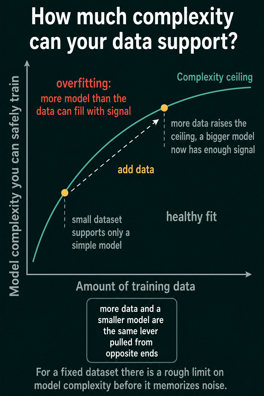
A curve of the model complexity a dataset can support against the amount of training data, with overfitting above the curve, a healthy fit below it, and an arrow showing that adding data raises the limit.

The curve in the picture flattens as data grows. Each extra batch of examples adds less new information than the one before it, because more of the new examples repeat what the model has already seen.

The formal version: sample complexity

Learning theory asks the same question with numbers. Sample complexity is the number of training examples needed to reach a target error with a target confidence. The target error is written $\varepsilon$, so a model that may be wrong on at most 5% of new inputs has $\varepsilon = 0.05$. A training set is a random draw, and an unlucky draw can mislead any learner, so the guarantee is allowed to fail with a small probability written $\delta$. The confidence is then $1 - \delta$.

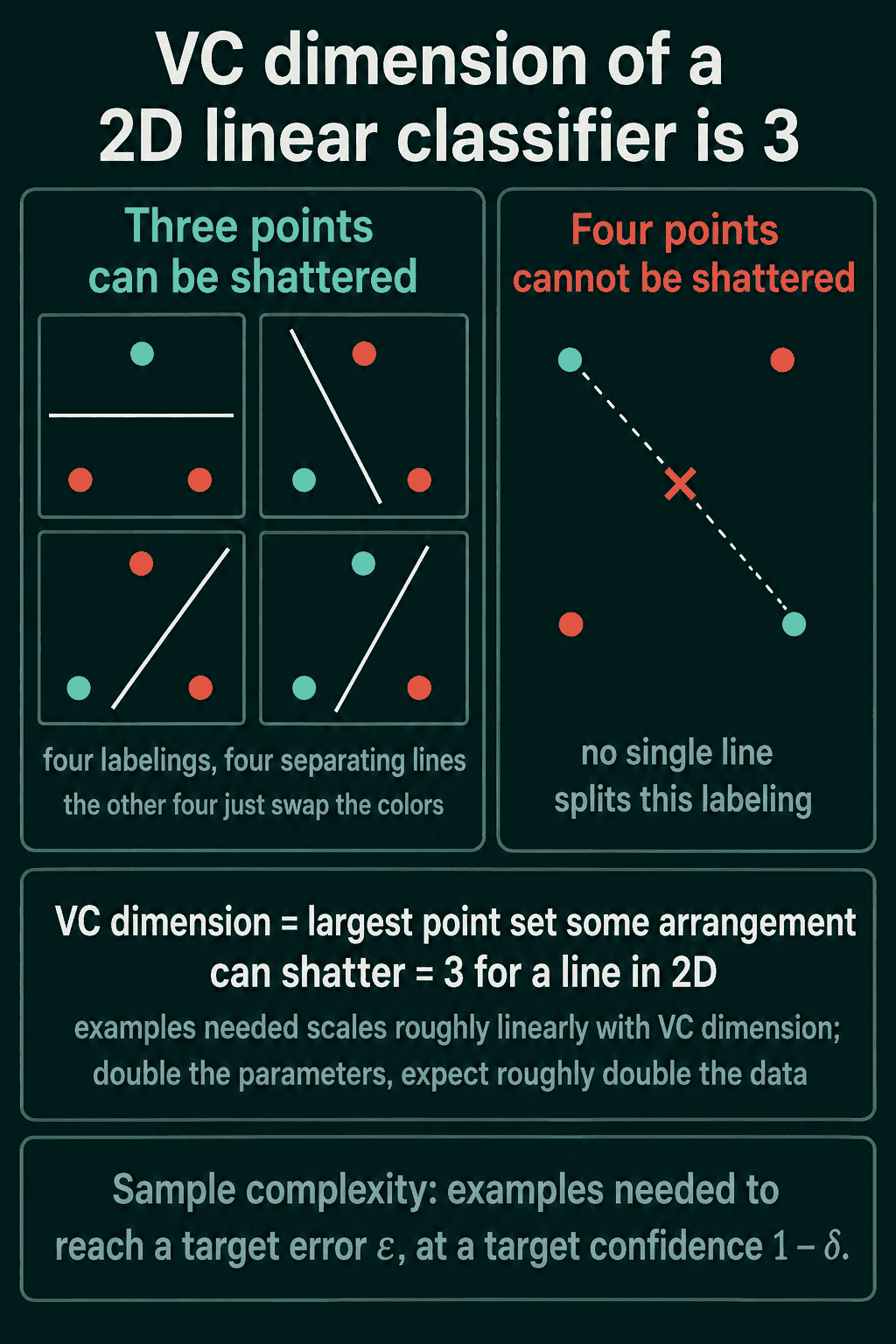
The question also needs a way to measure how expressive a model family is. The measure used here is the Vapnik-Chervonenkis dimension, or VC dimension. A model family shatters a set of points if, for every possible way of labeling those points with two classes, some model in the family produces exactly that labeling. The VC dimension is the size of the largest set of points the family can shatter.

A classifier that separates two classes with a straight line in 2D is a small example. Three points placed in a triangle can be shattered, because for each of the eight possible labelings some line puts the two classes on opposite sides. Four of the eight are the other four with the two classes swapped, so four lines cover all of them. Four points cannot be shattered. With four points at the corners of a square, labeling each diagonal pair as one class gives a labeling that no single line separates. So the VC dimension of a 2D linear classifier is 3.

For many model families the VC dimension is roughly proportional to the number of parameters, and the number of examples needed scales roughly linearly with it. Doubling the parameters roughly doubles the data the theory asks for.

Three points labeled in four ways, each split by a straight line, next to four points with a diagonal labeling that no single line splits, giving a VC dimension of 3 for a line in 2D.

What the bound says

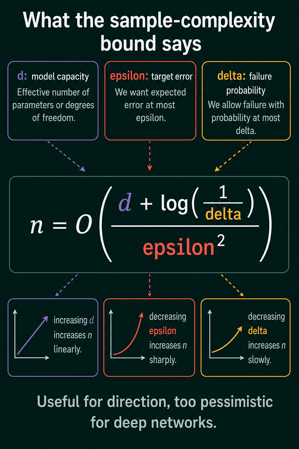
Let $n$ be the number of training examples and $d$ the VC dimension of the model family. In the general case, where no model in the family fits the data perfectly, the number of examples needed scales as

$$n = O!\left(\frac{d + \log(1/\delta)}{\varepsilon^2}\right)$$

The $O(\cdot)$ notation means "grows in proportion to", ignoring constant factors. The formula says the data requirement rises with model capacity, rises fast as the target error shrinks, and rises slowly as the allowed failure probability shrinks.

Each of the three terms can be read on its own:

Capacity enters through $d$. A more expressive model family needs more data, in direct proportion.
Error tolerance enters as $1/\varepsilon^2$. Halving the target error multiplies the data requirement by four.
Confidence enters as $\log(1/\delta)$. Going from a 5% failure probability to 0.5% adds about 2.3 to the numerator.

When some model in the family can fit the data perfectly, the $\varepsilon^2$ in the denominator becomes $\varepsilon$, and halving the target error only doubles the requirement.

The sample complexity bound with its three inputs labeled: model capacity d, target error epsilon, and failure probability delta, and a small plot of how the number of examples grows with each one.

Why nobody plugs numbers into the bound

The bound is a worst-case guarantee over every possible data distribution, and for a deep network it asks for far more data than the network needs in practice. Networks with millions of parameters are routinely trained on fewer examples than they have parameters and still do well on held-out data. Part of the reason is that parameter count overstates the capacity a trained network uses, since the optimizer and regularization push it toward a small subset of the functions it could represent.

The bound is still useful for direction. It puts math under two rules that hold up well in practice: larger models need more data, and each extra point of accuracy costs more data than the one before it.

How to tell whether more data would help

The practical test is a learning curve: train the same model on growing slices of the training set and record the validation loss for each slice. If validation loss is still falling at the largest slice, more data is likely to help. If it has flattened, more data of the same kind will not move it much, and the model or the features are the place to look.

The snippet trains a small network and a large one on 10, 40, 160, and 640 examples of a noisy sine curve.

1import torch
2import torch.nn as nn
3 
4def make_data(n, seed):
5    g = torch.Generator().manual_seed(seed)
6    x = torch.rand(n, 1, generator=g) * 6 - 3
7    y = torch.sin(x) + 0.3 * torch.randn(n, 1, generator=g)   # true curve plus noise
8    return x, y
9 
10x_val, y_val = make_data(2000, seed=1)                        # held-out examples
11 
12def fit(n_train, hidden, epochs=3000):
13    torch.manual_seed(0)
14    x, y = make_data(n_train, seed=0)
15    model = nn.Sequential(nn.Linear(1, hidden), nn.Tanh(), nn.Linear(hidden, 1))
16    opt = torch.optim.Adam(model.parameters(), lr=1e-2)
17    for _ in range(epochs):
18        opt.zero_grad()
19        loss = nn.functional.mse_loss(model(x), y)
20        loss.backward()
21        opt.step()
22    with torch.no_grad():
23        return (nn.functional.mse_loss(model(x), y).item(),
24                nn.functional.mse_loss(model(x_val), y_val).item())
25 
26for hidden in (4, 256):
27    for n_train in (10, 40, 160, 640):
28        train_loss, val_loss = fit(n_train, hidden)
29        print(f"hidden={hidden:3d}  examples={n_train:3d}  train={train_loss:.3f}  val={val_loss:.3f}")

1hidden=  4  examples= 10  train=0.024  val=0.188
2hidden=  4  examples= 40  train=0.056  val=0.101
3hidden=  4  examples=160  train=0.061  val=0.092
4hidden=  4  examples=640  train=0.095  val=0.089
5hidden=256  examples= 10  train=0.016  val=0.331
6hidden=256  examples= 40  train=0.050  val=0.108
7hidden=256  examples=160  train=0.062  val=0.091
8hidden=256  examples=640  train=0.094  val=0.088

With 10 examples, the large network's validation loss is 0.331 against 0.188 for the small one, so the extra capacity went into fitting noise. By 160 examples the two networks score about the same, and from 160 to 640 the validation loss barely moves. The noise added to the labels has variance $0.3^2 = 0.09$, which is the lowest validation loss any model can reach here, so both curves have flattened against that floor and more data would not help. To see a curve that is still falling, raise the noise or replace the sine with a harder function.

What to do when you cannot get more data

Use a smaller model. Fewer parameters bring the model back under the limit the dataset supports.
Regularize. Regularization is the set of techniques that hold a model back from fitting too closely, such as weight decay, dropout, and early stopping.
Start from a pretrained model. A model already trained on a large general dataset needs far fewer examples of the new task than one trained from random weights.
Augment the data. Data augmentation creates extra training examples by applying changes that keep the label the same, such as flipping or cropping an image.

Common mistakes

Counting rows instead of information. Ten thousand near-duplicate examples constrain a model about as much as the few distinct ones among them, and mislabeled examples add noise without adding signal.

Reading training loss alone. A training loss near zero on a small dataset says the model had enough capacity to memorize it, and the validation loss is the number that says whether it learned the pattern.

Adding input features without adding examples. Each new feature gives the model more to fit and spreads the same examples over a larger input space, which raises the amount of data needed.

Collecting more data after the learning curve has gone flat. Past that point the error is coming from the model, the features, or the noise in the labels.

The bias-variance tradeoff describes the same limit from the model's side: a model too simple for the pattern has high bias, and a model with more freedom than the data can constrain has high variance. The curse of dimensionality is the reason extra input features raise the data requirement, since the space the examples have to cover grows with each one. Double descent is the observation that test error can fall again once a model grows far past the point of fitting its training data exactly, which is one reason the classic bound overestimates what large networks need.

QuiddityML teaches model complexity against dataset size and sample complexity bounds as two concepts in the ML Foundation track, and the exercises ask which of two models is more likely to overfit a small dataset and what happens to the data requirement when the error tolerance is tightened.