1 October 2026 · 10 min read
How to read a loss curve: training vs validation loss
A loss curve is a plot of a model's loss over the course of training. This post explains how to plot training and validation loss together, what a healthy curve looks like, and what it means when validation loss goes up while training loss keeps going down.
A loss curve is a plot of a model's loss against training time. The loss is one number that measures how wrong the model's predictions are, and lower is better. Plotting it after each pass over the data shows whether the model is learning, whether it has stopped, and whether it is learning the training examples in a way that does not carry over to new ones. It is usually the first plot to look at when a training run gives a disappointing score.
Why two curves and not one
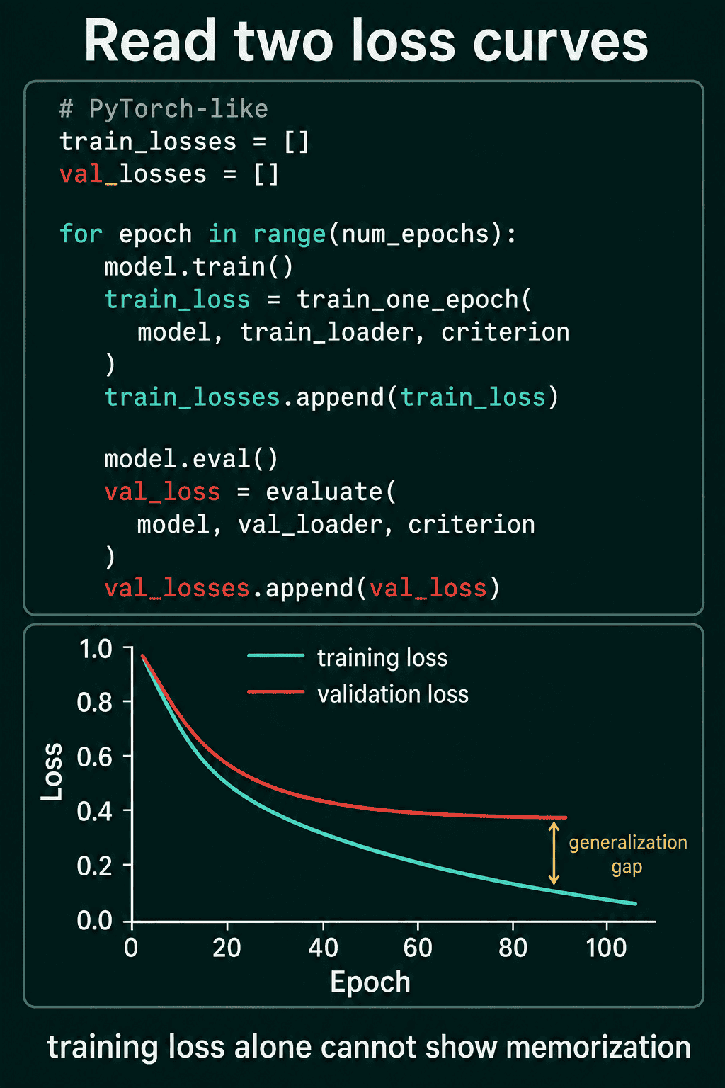
Training adjusts the model's weights to push the loss down on the training examples, so the training loss falls almost by construction. A model with enough weights can drive it close to zero by storing which training input goes with which label. That says nothing about inputs it has not seen.
The validation loss is the same loss measured on held-out examples that the model does not train on. It stands in for new data. The distance between the two curves, validation loss minus training loss, is called the generalization gap, and the training curve alone cannot show it.
Recording both takes two lists. After each epoch, one pass over the training data, the loop appends the training loss and the validation loss. model.train() and model.eval() switch layers such as dropout between their training and evaluation behaviour, and in the picture below criterion is the loss function.
Three runs on the same data
The script below produces three different curve shapes from one dataset. The data has 20 input features and a yes/no label that depends on a weighted sum of the features plus noise, so some labels cannot be predicted from the inputs. There are 200 training examples and 1,000 validation examples. The loss is cross-entropy, which for two classes is about 0.69 for a model that guesses 50/50.
The three runs are a linear model, a much larger network with two hidden layers of 256 units (an MLP), and that same large network with a learning rate 1,000 times smaller. The learning rate is the number that scales each weight update.
1import torch
2import torch.nn as nn
3
4torch.manual_seed(0)
5X = torch.randn(1200, 20)
6w_true = torch.randn(20)
7y = ((X @ w_true + 2.0 * torch.randn(1200)) > 0).long()   # labels with noise in them
8X_train, y_train, X_val, y_val = X[:200], y[:200], X[200:], y[200:]
9loss_fn = nn.CrossEntropyLoss()
10
11def fit(model, lr, num_epochs=200):
12    optimizer = torch.optim.Adam(model.parameters(), lr=lr)
13    history = {"train": [], "val": [], "val_acc": [], "val_conf": []}
14    for epoch in range(num_epochs):
15        model.train()
16        loss = loss_fn(model(X_train), y_train)
17        optimizer.zero_grad()
18        loss.backward()
19        optimizer.step()
20
21        model.eval()
22        with torch.no_grad():
23            val_logits = model(X_val)
24            history["train"].append(loss_fn(model(X_train), y_train).item())
25            history["val"].append(loss_fn(val_logits, y_val).item())
26            history["val_acc"].append((val_logits.argmax(dim=1) == y_val).float().mean().item())
27            history["val_conf"].append(torch.softmax(val_logits, dim=1).max(dim=1).values.mean().item())
28    return history
29
30def mlp():
31    return nn.Sequential(nn.Linear(20, 256), nn.ReLU(), nn.Linear(256, 256), nn.ReLU(), nn.Linear(256, 2))
32
33runs = {
34    "linear model, lr 0.01": (nn.Linear(20, 2), 0.01),
35    "large MLP, lr 0.001": (mlp(), 0.001),
36    "large MLP, lr 0.000001": (mlp(), 0.000001),
37}
38curves = {}
39for name, (model, lr) in runs.items():
40    h = curves[name] = fit(model, lr)
41    best = min(range(200), key=lambda e: h["val"][e])
42    print(name)
43    for e in [0, 9, 24, 49, 99, 199]:
44        print(f"  epoch {e + 1:3d}  train {h['train'][e]:.3f}  val {h['val'][e]:.3f}  gap {h['val'][e] - h['train'][e]:+.3f}")
45 print(f" lowest val loss {h['val'][best]:.3f} at epoch {best + 1}")1linear model, lr 0.01
2 epoch 1 train 0.708 val 0.706 gap -0.002
3 epoch 10 train 0.527 val 0.579 gap +0.052
4 epoch 25 train 0.404 val 0.489 gap +0.085
5 epoch 50 train 0.328 val 0.423 gap +0.094
6 epoch 100 train 0.277 val 0.367 gap +0.090
7 epoch 200 train 0.247 val 0.340 gap +0.093
8 lowest val loss 0.340 at epoch 200
9large MLP, lr 0.001
10 epoch 1 train 0.656 val 0.668 gap +0.012
11 epoch 10 train 0.366 val 0.440 gap +0.074
12 epoch 25 train 0.109 val 0.392 gap +0.283
13 epoch 50 train 0.006 val 0.670 gap +0.664
14 epoch 100 train 0.001 val 0.875 gap +0.874
15 epoch 200 train 0.000 val 1.003 gap +1.002
16 lowest val loss 0.353 at epoch 19
17large MLP, lr 0.000001
18 epoch 1 train 0.697 val 0.700 gap +0.003
19 epoch 10 train 0.697 val 0.700 gap +0.003
20 epoch 25 train 0.696 val 0.699 gap +0.003
21 epoch 50 train 0.695 val 0.699 gap +0.004
22 epoch 100 train 0.693 val 0.698 gap +0.005
23 epoch 200 train 0.688 val 0.695 gap +0.007
24 lowest val loss 0.695 at epoch 200The plot comes from the same curves dictionary, so this block runs after the one above.
1import matplotlib.pyplot as plt
2
3plt.style.use("dark_background")
4fig, axes = plt.subplots(1, 3, figsize=(15, 4.5), sharey=True)
5for ax, (name, h) in zip(axes, curves.items()):
6    ax.plot(range(1, 201), h["train"], color="#4fd1b5", linewidth=2.5, label="training loss")
7    ax.plot(range(1, 201), h["val"], color="#f0524f", linewidth=2.5, label="validation loss")
8    ax.set_title(name)
9    ax.set_xlabel("Epoch")
10    ax.grid(alpha=0.2)
11axes[0].set_ylabel("Loss")
12axes[0].legend()
13fig.tight_layout()
14fig.savefig("loss_curves.png", dpi=150)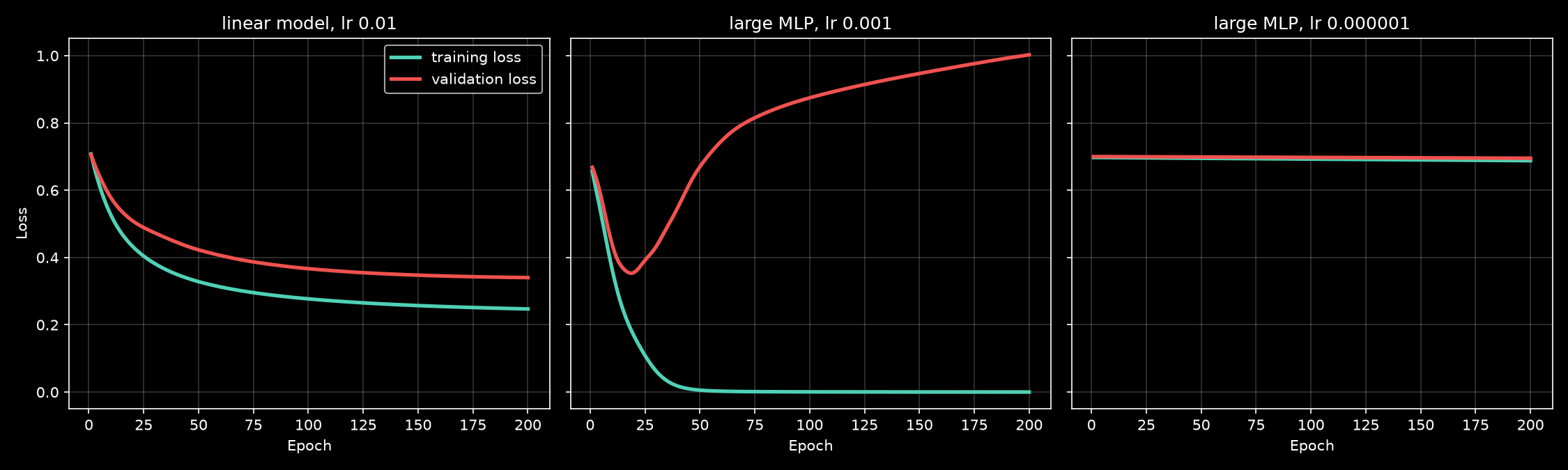
The next three sections read these three panels from left to right.
What a healthy curve looks like
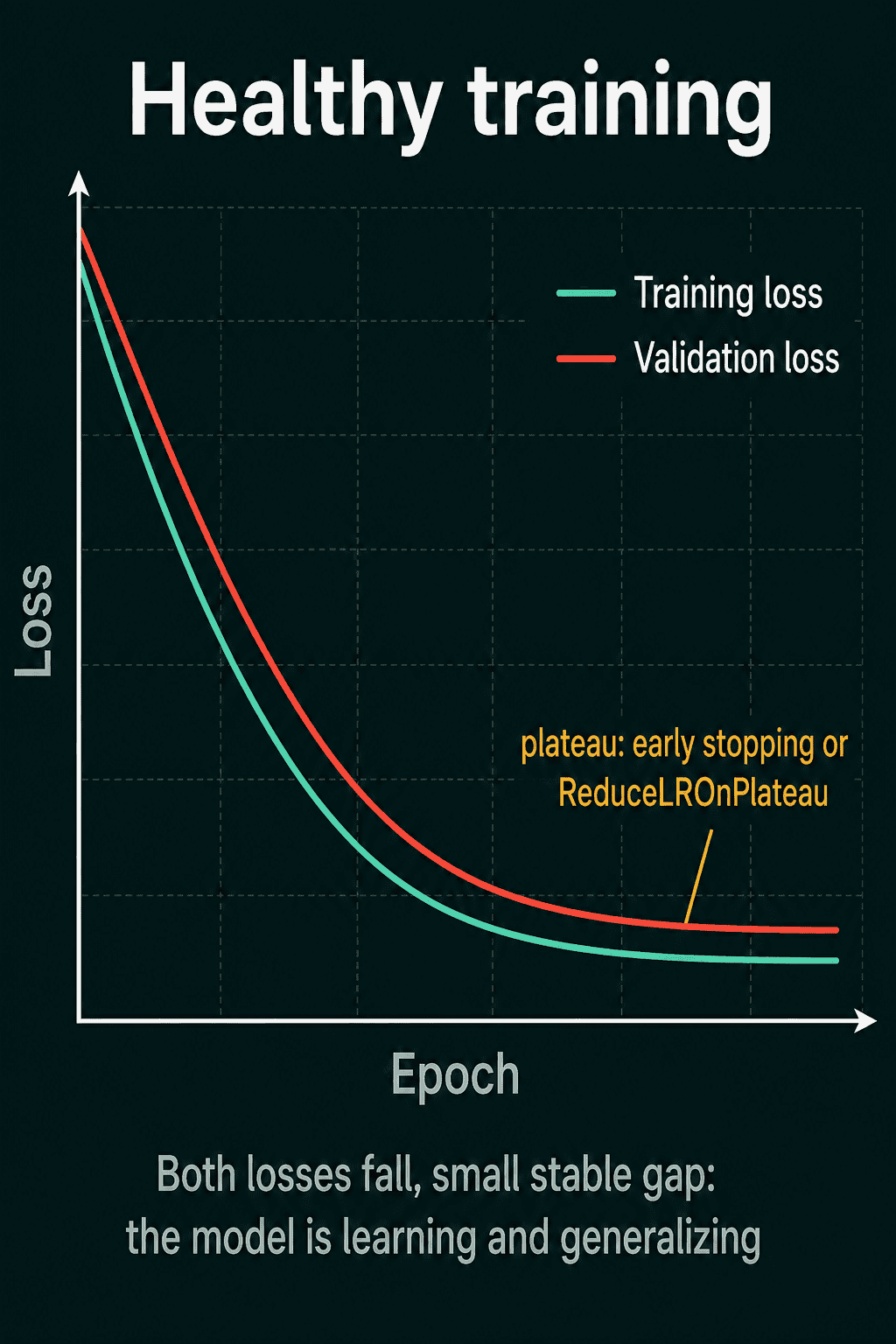
In the left panel both losses fall quickly, slow down and flatten. The validation loss sits a little above the training loss, and the gap stops growing: it is 0.094 at epoch 50 and 0.093 at epoch 200. The lowest validation loss is at the last epoch, so no earlier point in training was better.
That is the pattern to compare other runs against.
- Both losses go down.
- The validation loss follows the training loss with a small gap that stays about the same size.
- The curves flatten as the model runs out of things to learn from this data with this setup.
- The validation loss is a little higher than the training loss, which is expected, since the weights were fit to the training examples.
The flat stretch at the end is called a plateau. Two common ways to handle it are early stopping, which ends training once the validation loss has stopped improving and keeps the weights from its lowest point, and ReduceLROnPlateau, a PyTorch learning rate schedule that lowers the learning rate when the validation loss stalls.
Validation loss goes up while training loss goes down
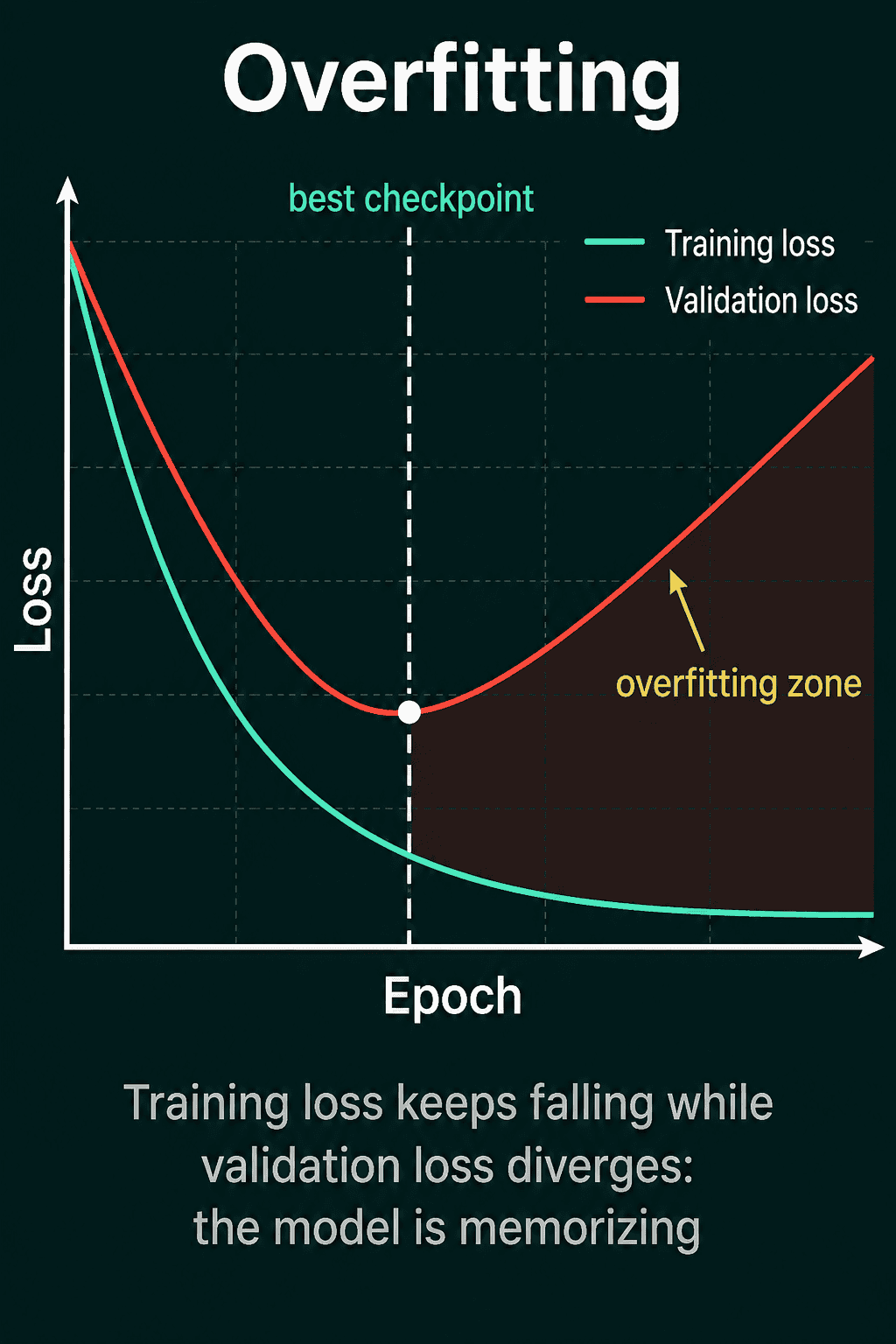
In the middle panel the training loss falls to 0.006 by epoch 50 and to 0.000 by epoch 200. The validation loss reaches its lowest value, 0.353, at epoch 19 and then rises to 1.003. The gap grows from 0.074 at epoch 10 to 1.002 at the end.
This is overfitting. After epoch 19 the network keeps lowering the training loss by fitting the noise in the 200 training labels, which has no pattern that could hold for the validation examples. Each further epoch makes it better on the training set and worse on held-out data.
The model to keep is the one from the lowest point of the validation curve. Saving the weights each time the validation loss reaches a new low gives a best checkpoint, a file holding the weights from that epoch, and everything to the right of it on the plot is training that made the model worse.
Fixes work on the gap: more training data, a smaller model, regularization such as weight decay or dropout, or stopping at the best checkpoint. The linear model in the left panel is the "smaller model" fix applied to this dataset. It ends at a validation loss of 0.340, lower than the best epoch of the large network.
Both losses stay high
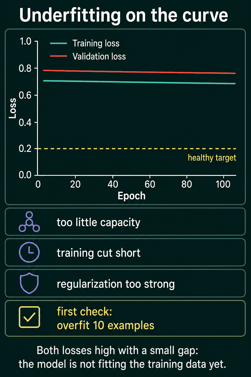
In the right panel the training loss moves from 0.697 to 0.688 over 200 epochs and the validation loss stays next to it. Both are close to 0.69, the loss of a 50/50 guess. The gap is tiny, and that is not good news here, because a small gap only says the model does equally badly on both sets.
This is underfitting: the model has not fit the training data. The run above underfits because the learning rate is too small for 200 epochs to move the weights far. The other common causes are a model with too little capacity, meaning too few weights to represent the pattern, and regularization set so strong that it holds the weights back.
A quick test separates "cannot learn" from "has not learned yet". Train on about 10 examples and check that the training loss goes to near zero. A model and training loop that cannot memorize 10 examples have a bug or a setting that is far off, and more data will not fix that.
What the training loss alone tells you about the learning rate
The shape of the training loss on its own says a lot about the learning rate, before the validation curve comes into it. Here the horizontal axis is usually the iteration, one weight update, instead of the epoch.
- Too high: the loss jumps up and down, grows, or turns into
nan. Each update overshoots. - About right: the loss drops quickly at first and then flattens.
- Too low: the loss goes down in a nearly straight, shallow line, as in the right panel above.
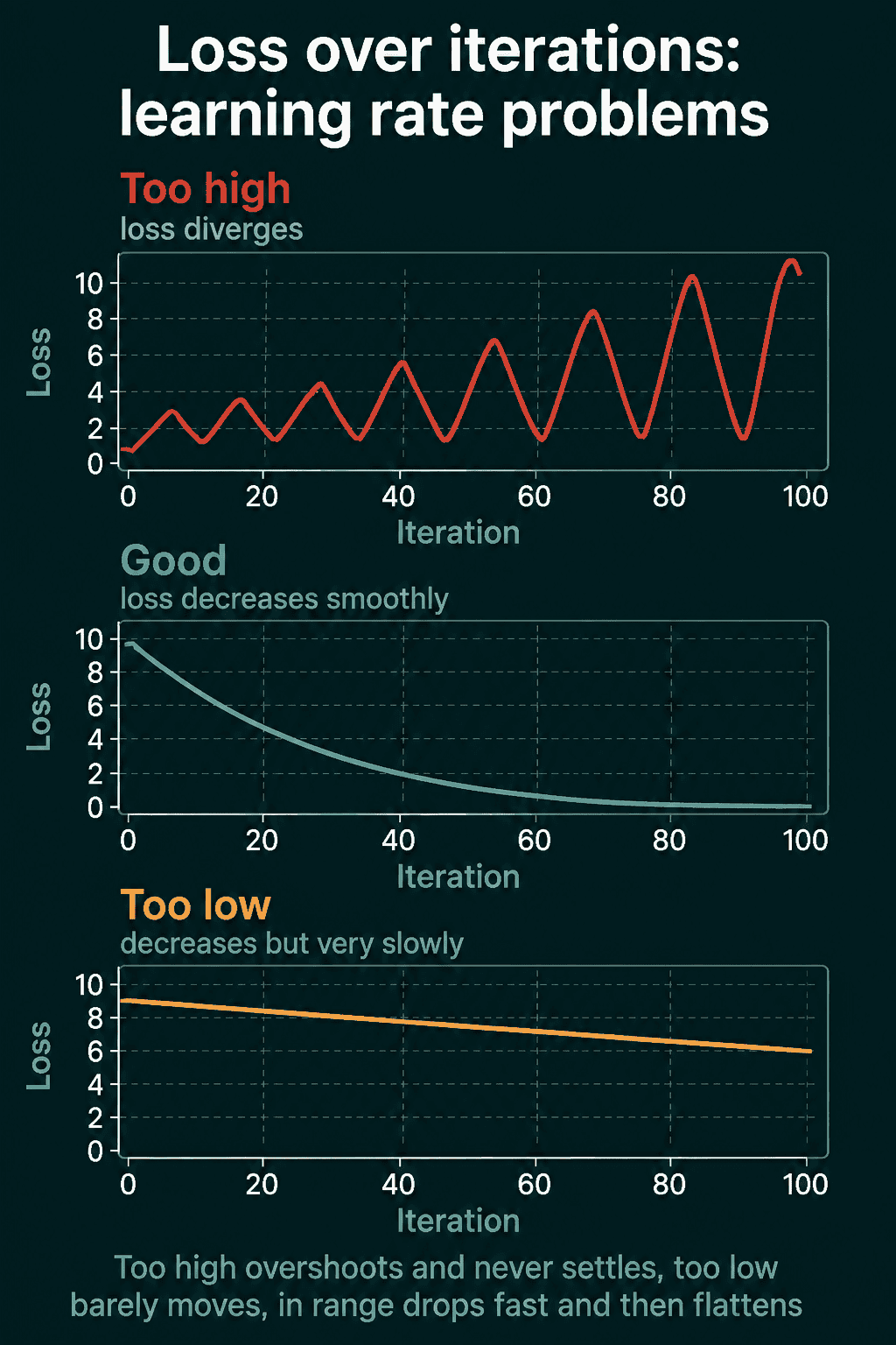
What is a learning rate? goes through these three cases and how to pick a starting value.
A table of shapes
| Shape | What it usually means | First thing to try |
|---|---|---|
| Both fall, small steady gap | Healthy | Train until the plateau |
| Train falls, validation rises | Overfitting | Keep the best checkpoint |
| Both high and flat | Underfitting | Overfit 10 examples |
| Loss jumps or grows | Learning rate too high | Divide it by 10 |
| Slow straight decline | Learning rate too low | Multiply it by 10 |
| Validation below training | Dropout, or timing | Evaluate both in eval mode |
The last row has two ordinary causes. Dropout and similar layers are active while the training loss is computed and switched off for validation, so the training loss is measured on a model with part of its units zeroed out. The training loss is also often averaged over the batches of an epoch, while the weights were still improving, and the validation loss is measured at the end of it. The script above avoids both by recomputing the training loss in eval mode after each update. A validation loss far below the training loss is worth a closer look at how the data was split.
What a loss curve does not show
A loss curve averages over all the examples, so some problems do not appear in it.
Accuracy can move differently from the loss. Accuracy counts whether the top prediction is correct. Cross-entropy loss also depends on how much probability the model gave the correct class, and it grows without limit as that probability goes to zero. A model that becomes very sure of its wrong answers can keep nearly the same accuracy while its loss climbs.
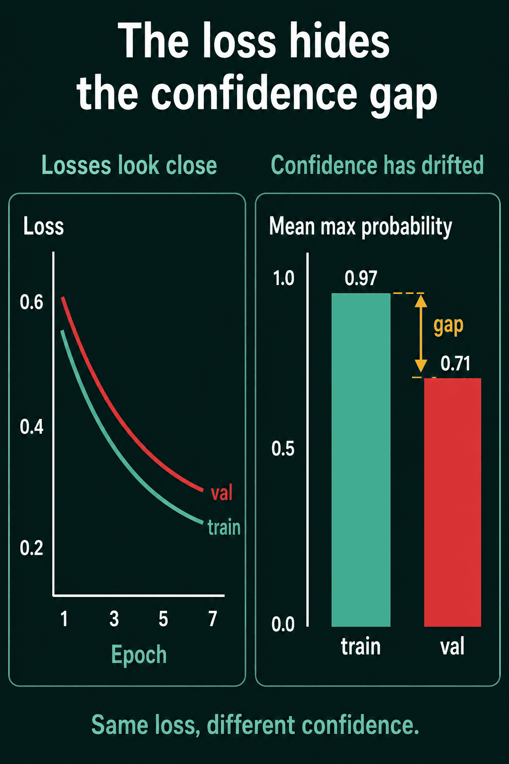
Confidence can drift. The model's confidence in a prediction is the highest probability it assigns to any class. Averaging that over a dataset gives one number, the mean max probability, computed with probs.max(dim=1).values.mean(). The highest probability is used instead of the probability of the correct class because it also captures predictions that are confident and wrong.
The large network from the middle panel shows both effects. This block continues from the first script.
1h = curves["large MLP, lr 0.001"]
2for e in [18, 199]:
3    print(f"epoch {e + 1:3d}  val loss {h['val'][e]:.3f}  val accuracy {h['val_acc'][e]:.3f}  mean confidence {h['val_conf'][e]:.3f}")
4
5model = runs["large MLP, lr 0.001"][0]             # the weights after epoch 200
6with torch.no_grad():
7    logits = model(X_val)
8    per_example = nn.functional.cross_entropy(logits, y_val, reduction="none")
9    wrong = logits.argmax(dim=1) != y_val
10print(f"wrong predictions: {wrong.float().mean():.1%} of examples, {per_example[wrong].sum() / per_example.sum():.1%} of the loss")1epoch 19 val loss 0.353 val accuracy 0.850 mean confidence 0.849
2epoch 200 val loss 1.003 val accuracy 0.805 mean confidence 0.960Between epoch 19 and epoch 200 the validation loss nearly triples, while validation accuracy falls by only 4.5 points, from 85.0% to 80.5%. At epoch 19 the model's mean confidence of 0.849 matches its accuracy of 0.850. At epoch 200 it is 96% confident on average and right 80.5% of the time. The last line splits the epoch-200 loss by example: the 19.5% of validation examples the model gets wrong account for 97.8% of the loss, because each of them is a wrong answer given with high confidence.
The picture below shows the related case where the two loss curves look close and the confidence still differs between the sets: 0.97 on the training data against 0.71 on the validation data. Logging the mean max probability on both sets next to the losses catches this.
Common mistakes
- Plotting only the training loss. A falling training loss looks the same for a model that is learning a pattern and one that is memorizing.
- Reading one noisy point. With small batches or a small validation set the curve jitters. Look at the trend over several epochs, or plot a moving average, before deciding the validation loss has turned.
- Comparing losses computed in different modes. A training loss with dropout on and a validation loss with it off are not measuring the same model.
- Keeping the last epoch. In the middle panel the last epoch has a validation loss of 1.003 and the best one 0.353.
- Comparing curves across loss functions or datasets. A loss of 0.3 with cross-entropy and 0.3 with mean squared error are different quantities. Compare runs that share the loss and the validation set.
- Treating the validation loss as the final score. The best epoch was chosen using it, so the number to report comes from a separate test set.
Related concepts
Overfitting and underfitting covers the causes and fixes behind the two failing shapes. The bias-variance tradeoff explains why a model that is too small and one that is too large fail in different ways. The train, validation and test split is where the validation curve's data comes from. Saving and resuming training shows how to write the best checkpoint. When the loss does not move at all, the loss-not-decreasing checklist goes through the usual causes.
QuiddityML teaches reading a loss curve as a concept in Unit 4 of the ML Foundation track, with questions such as whether a validation loss that sits 0.05 above the training loss for the whole run is a problem, and the spaced review brings the curve shapes back until they are quick to recognize (quiddityml.com).