By Sagi Shaier · 8 October 2026 · 7 min read

Solving systems of linear equations with Gaussian elimination

How to solve a 2x2 and a 3x3 system of equations by hand with row operations, how to tell from the reduced rows whether there is one solution, none, or infinitely many, and the same steps in PyTorch.

A system of linear equations is a set of equations that share the same unknowns, where each unknown is only multiplied by a number and added. Gaussian elimination is a common way to solve one by hand: add and scale the equations to cancel unknowns one at a time until each value can be read off. The same question shows up when a model or an algorithm needs the input that produces a known output.

Writing a system as Ax = b

A matrix times a vector, $A\mathbf{x}$, takes an input vector $\mathbf{x}$ and returns an output vector. A system of linear equations asks the reverse question: given the matrix $A$ and an output $\mathbf{b}$, which input $\mathbf{x}$ produces it?

$$A\mathbf{x} = \mathbf{b}$$

Each row of $A$ holds the numbers multiplying the unknowns in one equation, and the matching entry of $\mathbf{b}$ is that equation's right-hand side. Two equations in two unknowns,

$$2x_1 + x_2 = 5$$

$$x_1 - x_2 = 1$$

are $A\mathbf{x} = \mathbf{b}$ with $A = \begin{bmatrix} 2 & 1 \ 1 & -1 \end{bmatrix}$ and $\mathbf{b} = \begin{bmatrix} 5 \ 1 \end{bmatrix}$.

Solving a 2x2 system by elimination

Adding the two equations cancels $x_2$, because one has $+x_2$ and the other has $-x_2$:

$$(2x_1 + x_2) + (x_1 - x_2) = 5 + 1$$

which leaves $3x_1 = 6$, so $x_1 = 2$. Putting $x_1 = 2$ back into the second equation gives $2 - x_2 = 1$, so $x_2 = 1$.

The same work is usually written as an augmented matrix, which is $A$ with $\mathbf{b}$ added as an extra column and a bar between them:

$$\left[\begin{array}{cc|c} 2 & 1 & 5 \ 1 & -1 & 1 \end{array}\right]$$

Adding row 2 to row 1 turns the top row into $[,3\ \ 0 \mid 6,]$, which reads back as $3x_1 = 6$. Working on rows of numbers instead of written equations is what lets the method scale to larger systems.

The three row operations

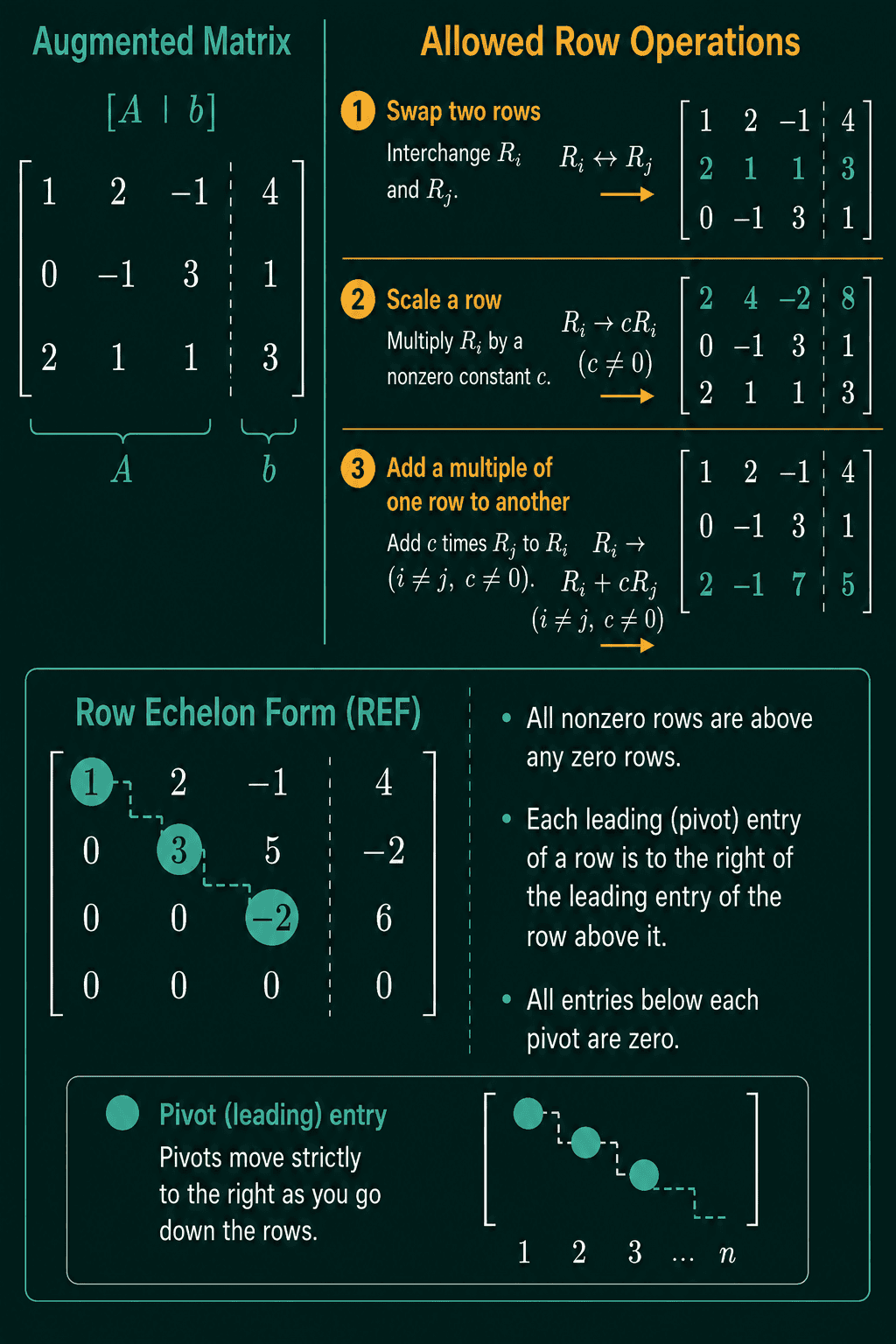
Every move in Gaussian elimination is one of three operations on the rows of the augmented matrix, and none of them changes which $\mathbf{x}$ solves the system:

Swap two rows.
Scale a row by a number that is not zero.
Add a multiple of one row to another row.

The goal is a staircase shape. A pivot is the first nonzero entry in a row once you are done working on that row. A matrix is in row echelon form when each pivot sits strictly to the right of the pivot in the row above, so every entry below the staircase is 0. Back substitution finishes the job: the bottom row has one unknown left, so solve it, then push that value up into the row above, and keep going to the top.

The augmented matrix with rows (1, 2, minus 1 | 4), (0, minus 1, 3 | 1) and (2, 1, 1 | 3), the result of swapping two rows, scaling a row by 2, and adding 2 times row 2 to row 3, and an example of row echelon form with pivots stepping to the right

A 3x3 example, step by step

Take three equations in three unknowns:

$$x_1 + 2x_2 + x_3 = 8$$

$$2x_1 + x_2 - x_3 = 1$$

$$3x_1 - x_2 + 2x_3 = 7$$

As an augmented matrix:

$$\left[\begin{array}{ccc|c} 1 & 2 & 1 & 8 \ 2 & 1 & -1 & 1 \ 3 & -1 & 2 & 7 \end{array}\right]$$

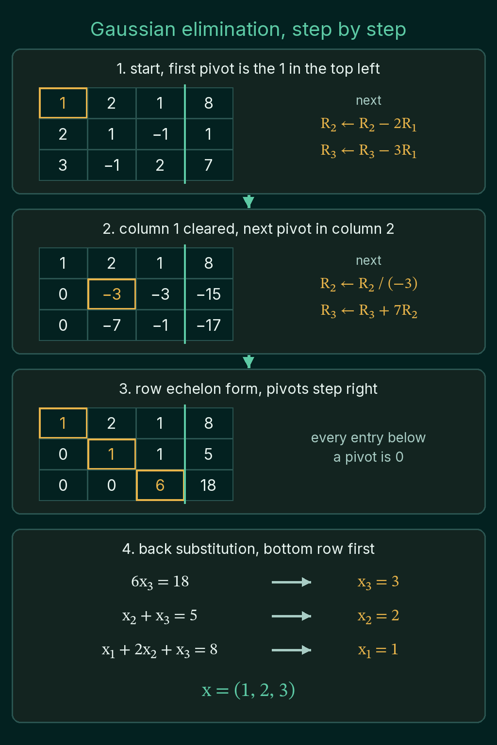
The first pivot is the 1 in the top left, and the job is to make every entry under it 0. Write $R_1$, $R_2$, $R_3$ for the three rows, and $R_2 \leftarrow R_2 - 2R_1$ for "replace row 2 with row 2 minus twice row 1". That operation turns row 2 into $[,0\ \ -3\ \ -3 \mid -15,]$, and $R_3 \leftarrow R_3 - 3R_1$ turns row 3 into $[,0\ \ -7\ \ -1 \mid -17,]$.

Column 2 is next. Scaling row 2 first keeps the numbers small: $R_2 \leftarrow R_2 / (-3)$ gives $[,0\ \ 1\ \ 1 \mid 5,]$, so the second pivot is 1. Then $R_3 \leftarrow R_3 + 7R_2$ clears the entry below it and turns row 3 into $[,0\ \ 0\ \ 6 \mid 18,]$:

$$\left[\begin{array}{ccc|c} 1 & 2 & 1 & 8 \ 0 & 1 & 1 & 5 \ 0 & 0 & 6 & 18 \end{array}\right]$$

That is row echelon form, with pivots 1, 1 and 6 stepping one column to the right each row.

Back substitution reads the answer off from the bottom up. The bottom row says $6x_3 = 18$, so $x_3 = 3$. The middle row says $x_2 + x_3 = 5$, so $x_2 = 2$. The top row says $x_1 + 2x_2 + x_3 = 8$, so $x_1 = 8 - 4 - 3 = 1$. The solution is $\mathbf{x} = (1, 2, 3)$, and putting it back into the three original equations checks out.

Gaussian elimination on the system above in four steps: clearing column 1 under the first pivot, scaling row 2 and clearing column 2, the row echelon form with pivots 1, 1 and 6, and back substitution giving x3 = 3, x2 = 2, x1 = 1

The swap operation did not come up here. It is needed when the entry you want as a pivot is 0: swap that row with a lower row that has a nonzero entry in the same column, then carry on. If no lower row has one, that column gets no pivot, and the system does not have exactly one solution.

The three possible outcomes

A system of linear equations ends in one of three ways:

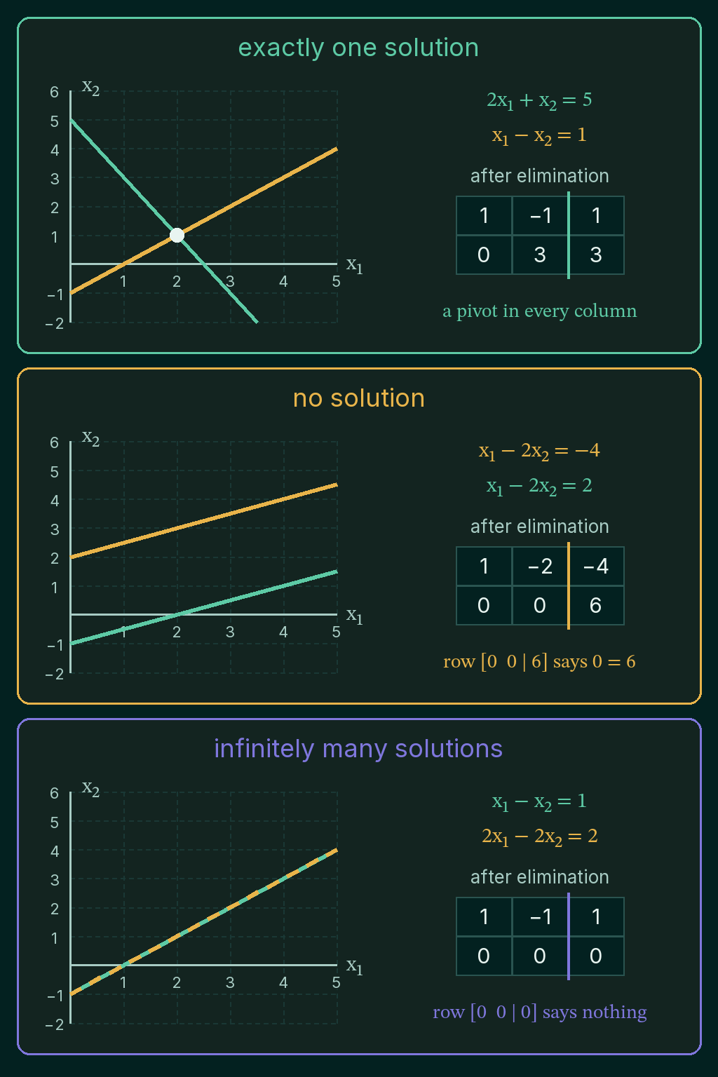
Exactly one solution. The equations pin $\mathbf{x}$ down to a single point. In 2D, the two lines cross once.
No solution. The equations contradict each other. In 2D, the two lines are parallel and never meet.
Infinitely many solutions. The equations do not hold enough independent information to pin $\mathbf{x}$ down. In 2D, both equations describe the same line.

Elimination shows which case you are in. A row that ends up as $[,0\ \ 0 \mid c,]$ with $c$ not zero says $0 = c$, which is impossible, so there is no solution. A row that ends up as $[,0\ \ 0 \mid 0,]$ says $0 = 0$, so that equation added nothing, and the remaining equations may leave a whole family of solutions.

Three panels: lines 2x1 + x2 = 5 and x1 minus x2 = 1 crossing at (2, 1) with a pivot in every column after elimination, the parallel lines x1 minus 2x2 = minus 4 and x1 minus 2x2 = 2 whose eliminated row is 0 0 | 6, and the same line written twice as x1 minus x2 = 1 and 2x1 minus 2x2 = 2 whose eliminated row is 0 0 | 0

For a square matrix $A$, whether every $\mathbf{b}$ has exactly one solution depends only on $A$. When $A$ fails that test, the particular $\mathbf{b}$ decides between no solution and infinitely many.

Gaussian elimination in PyTorch

The function below runs the same steps on a tensor: build the augmented matrix, clear each column under its pivot (swapping rows when the pivot spot holds 0), then back-substitute. It skips the scaling step, so its row echelon form has $-3$ where the hand version has 1, and it reaches the same answer. torch.linalg.solve is the built-in solver to use in real code.

1import torch
2 
3def gaussian_elimination(A, b):
4    M = torch.cat([A, b.unsqueeze(1)], dim=1)       # augmented matrix [A | b]
5    n = A.shape[0]
6    for col in range(n):
7        # swap in a row with a nonzero entry if the pivot spot holds 0
8        nonzero = (M[col:, col] != 0).nonzero()
9        if len(nonzero) == 0:
10            raise ValueError(f"no pivot in column {col}")
11        r = col + nonzero[0].item()
12        M[[col, r]] = M[[r, col]]
13        for row in range(col + 1, n):                # clear the entries below the pivot
14            M[row] -= (M[row, col] / M[col, col]) * M[col]
15    print(M)
16    x = torch.zeros(n)
17    for row in reversed(range(n)):                   # back substitution, bottom row first
18        x[row] = (M[row, -1] - M[row, row + 1:n] @ x[row + 1:]) / M[row, row]
19    return x
20 
21A = torch.tensor([[1., 2., 1.],
22                  [2., 1., -1.],
23                  [3., -1., 2.]])
24b = torch.tensor([8., 1., 7.])
25print(gaussian_elimination(A, b))
26print(torch.linalg.solve(A, b))
27 
28# the 2x2 system 2x1 + x2 = 5, x1 - x2 = 1
29print(torch.linalg.solve(torch.tensor([[2., 1.], [1., -1.]]), torch.tensor([5., 1.])))
30 
31# two equations for the same line: no single solution
32try:
33    torch.linalg.solve(torch.tensor([[1., -1.], [2., -2.]]), torch.tensor([1., 2.]))
34except RuntimeError as e:
35    print(str(e).splitlines()[0])

1tensor([[  1.,   2.,   1.,   8.],
2        [  0.,  -3.,  -3., -15.],
3        [  0.,   0.,   6.,  18.]])
4tensor([1., 2., 3.])
5tensor([1., 2., 3.])
6tensor([2., 1.])
7torch.linalg.solve: The solver failed because the input matrix is singular.

The last call fails because $x_1 - x_2 = 1$ and $2x_1 - 2x_2 = 2$ describe the same line, so there is no single answer to return. When torch.linalg.solve raises this error, the system has either no solution or infinitely many, and the next step is to check the rows of $A$ for one that is a multiple or combination of the others.

Common mistakes

Forgetting the right-hand side. A row operation has to be applied to the $\mathbf{b}$ column too, or the augmented matrix no longer describes the same system.
Scaling a row by 0. That wipes out an equation, so it is not one of the allowed operations.
Reading a $[,0\ \ 0 \mid 0,]$ row as "no solution". It means that equation was redundant. The impossible row is $[,0\ \ 0 \mid c,]$ with $c$ not zero.
Stopping before back substitution. Row echelon form only gives the last unknown directly, and the rest come from working upward.

Matrix multiplication, which defines what $A\mathbf{x}$ means, is covered in matrix multiplication explained. The determinant and inverse, which decide in advance whether a square system has exactly one solution, are in determinant, inverse and trace explained.

QuiddityML teaches systems of linear equations and Gaussian elimination as their own concept in the linear algebra part of the Math track, and the exercises include putting the elimination steps for the 3x3 system above in order and writing a solve_system function with torch.linalg.solve.