By Sagi Shaier · 8 October 2026 · 7 min read

Determinant, trace and inverse: when a matrix is singular

How to compute a determinant for 2x2 and 3x3 matrices, what a zero determinant means for inverting a matrix and solving equations, why torch.linalg.solve beats torch.linalg.inv in code, and where the trace shows up.

The determinant of a square matrix is a single number that says how much the matrix scales area (in 2D) or volume (in 3D) when it transforms space. A determinant of 0 means the matrix squashes space into fewer dimensions, which makes it singular: it has no inverse, so no matrix can undo it.

What the determinant measures

A matrix $A$ transforms vectors: $A\mathbf{x}$ takes a vector $\mathbf{x}$ and returns a new one. Applying $A$ to every corner of the unit square (the square with corners $(0, 0)$, $(1, 0)$, $(1, 1)$ and $(0, 1)$, which has area 1) turns it into a new shape, and the determinant, written $\det(A)$ or $|A|$, is the area of that shape:

$\det(A) = 2$ means the transformation doubles area.
$\det(A) = 1$ means area is unchanged, even if the shape is rotated or slanted.
A negative determinant means the transformation also flips the shape over, like a mirror image, and the size of the number is still the area factor.
$\det(A) = 0$ means the square is squashed into a line or a point, so its area is 0.

The zero case is the one with consequences. Once a plane is squashed onto a line, many different inputs land on the same output, and there is no way to tell from the output which input it came from.

For a $2 \times 2$ matrix the determinant has a direct formula:

$$\det\begin{bmatrix} a & b \ c & d \end{bmatrix} = ad - bc$$

For $A$ with rows $(2, 1)$ and $(0, 1)$, that gives $2 \cdot 1 - 1 \cdot 0 = 2$, and the unit square becomes a slanted shape of area 2. For the matrix with rows $(1, 2)$ and $(2, 4)$, it gives $1 \cdot 4 - 2 \cdot 2 = 0$, and every corner of the square lands on the line through $(1, 2)$.

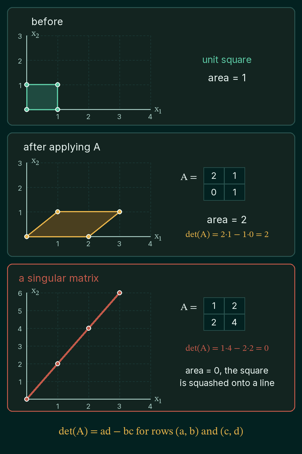
The unit square with area 1, the same square after the matrix with rows (2, 1) and (0, 1) turned into a parallelogram with corners (0, 0), (2, 0), (3, 1), (1, 1) and area 2, and the matrix with rows (1, 2) and (2, 4) squashing the square onto a line from (0, 0) to (3, 6) with determinant 0

Three properties follow from reading the determinant as an area factor. Applying two transformations in a row multiplies their factors, so $\det(AB) = \det(A)\det(B)$. Transposing a matrix (swapping its rows and columns) leaves the determinant unchanged, $\det(A^\top) = \det(A)$. And undoing a transformation undoes its scaling, $\det(A^{-1}) = 1 / \det(A)$, which only makes sense when $\det(A) \neq 0$.

Determinants of 3x3 matrices and larger

Cofactor expansion builds the determinant of an $n \times n$ matrix out of determinants of $(n-1) \times (n-1)$ matrices. Expanding along the top row:

$$\det(A) = \sum_{j=1}^{n} (-1)^{1+j} a_{1j} \det(M_{1j})$$

Here $a_{1j}$ is the entry in row 1 and column $j$, and $M_{1j}$ is the minor, the smaller matrix left after deleting row 1 and column $j$. The factor $(-1)^{1+j}$ alternates the sign across the row: plus, minus, plus. For a $3 \times 3$ matrix every minor is $2 \times 2$, so $ad - bc$ handles each one.

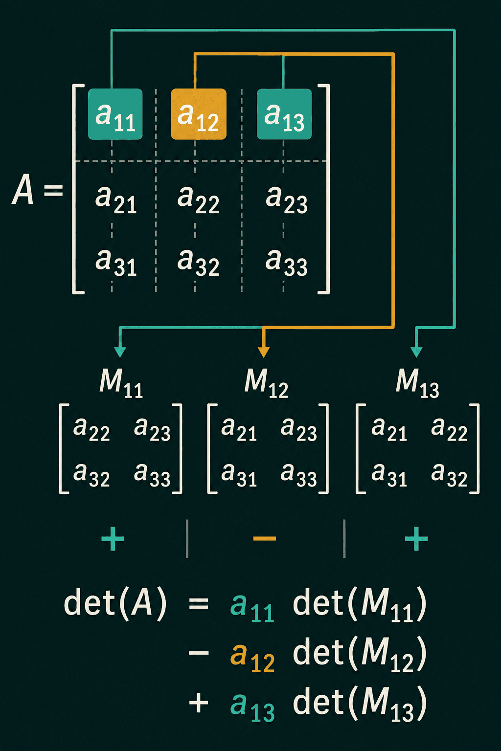
Cofactor expansion of a 3 by 3 matrix along its top row: deleting row 1 and each column in turn leaves the minors M11, M12 and M13, combined as a11 det(M11) minus a12 det(M12) plus a13 det(M13)

Take

$$A = \begin{bmatrix} 2 & 1 & 3 \ 0 & 4 & 1 \ 5 & 2 & 6 \end{bmatrix}$$

The three minors have determinants $4 \cdot 6 - 1 \cdot 2 = 22$, $0 \cdot 6 - 1 \cdot 5 = -5$ and $0 \cdot 2 - 4 \cdot 5 = -20$. With the plus, minus, plus signs:

$$\det(A) = 2(22) - 1(-5) + 3(-20) = -11$$

The expansion works along any row or column, with the sign of entry $a_{ij}$ given by $(-1)^{i+j}$, so picking the row or column with the most zeros saves work. The number of smaller determinants grows quickly with size, which is why torch.linalg.det computes determinants with elimination instead.

The inverse: undoing a transformation

If $A$ turns $\mathbf{x}$ into $\mathbf{b}$, the inverse $A^{-1}$ is the matrix that turns $\mathbf{b}$ back into $\mathbf{x}$. It satisfies

$$A^{-1}A = AA^{-1} = I$$

where $I$ is the identity matrix, with 1s on the diagonal and 0s elsewhere, which leaves every vector unchanged.

The inverse exists exactly when $\det(A) \neq 0$. A matrix with $\det(A) = 0$ is called singular and has no inverse, because the squashing step threw information away. A matrix with $\det(A) \neq 0$ is invertible, also called non-singular.

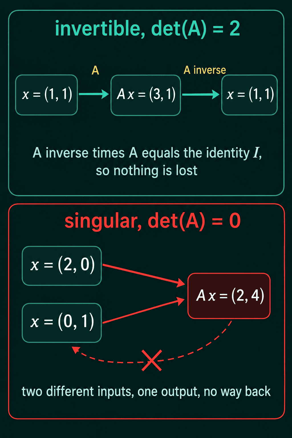
Top: the invertible matrix with determinant 2 sends (1, 1) to (3, 1), and its inverse sends (3, 1) back to (1, 1). Bottom: a singular matrix with determinant 0 sends both (2, 0) and (0, 1) to (2, 4), so there is no way back

The top half of that picture uses the same matrix as before, with rows $(2, 1)$ and $(0, 1)$, and the bottom half uses the singular matrix with rows $(1, 2)$ and $(2, 4)$, which sends $(2, 0)$ and $(0, 1)$ to the same output $(2, 4)$.

For a $2 \times 2$ matrix the inverse has a formula, with the determinant in the denominator:

$$\begin{bmatrix} a & b \ c & d \end{bmatrix}^{-1} = \frac{1}{ad - bc}\begin{bmatrix} d & -b \ -c & a \end{bmatrix}$$

When $ad - bc = 0$ there is nothing to divide by, which is the same fact seen from the formula.

Three algebra rules come up when simplifying expressions by hand. Inverting a product reverses the order of its factors, $(AB)^{-1} = B^{-1}A^{-1}$. Inverting and transposing can be done in either order, $(A^\top)^{-1} = (A^{-1})^\top$. And inverting twice returns the original matrix, $(A^{-1})^{-1} = A$.

Solving with the inverse, and why code uses solve instead

With $A^{-1}$ in hand, the solution of $A\mathbf{x} = \mathbf{b}$ is

$$\mathbf{x} = A^{-1}\mathbf{b}$$

In code, torch.linalg.solve(A, b) is preferred over torch.linalg.inv(A) @ b. Both give the same answer in exact math, and computing the full inverse first is slower and loses more accuracy to floating-point rounding.

Checking for a singular matrix in code needs care too. Floating-point arithmetic rarely lands on exactly 0.0, so a matrix that is singular on paper can report a determinant like 1e-17. Compare the absolute value against a small tolerance instead of testing for 0. That test only works for small matrices: a large determinant is a product of many factors, so it can be tiny for a matrix that is perfectly invertible. For large matrices, torch.linalg.matrix_rank is the better check.

The trace

The trace of a square matrix is the sum of its diagonal entries, the ones running from the top left to the bottom right:

$$\text{tr}(A) = \sum_i A_{ii}$$

The trace adds across sums, $\text{tr}(A + B) = \text{tr}(A) + \text{tr}(B)$, and it stays the same when a product is rotated: $\text{tr}(ABC) = \text{tr}(BCA) = \text{tr}(CAB)$. That second rule holds even though $AB$ and $BA$ are usually different matrices.

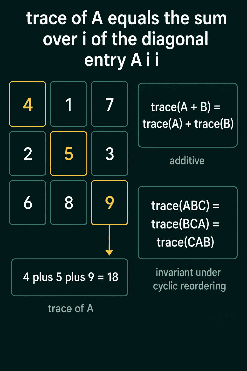
A 3 by 3 matrix with diagonal entries 4, 5 and 9 highlighted, summing to a trace of 18, next to the rules trace(A + B) = trace(A) + trace(B) and trace(ABC) = trace(BCA) = trace(CAB)

The trace mostly shows up inside derivations rather than everyday code. For example, $\text{tr}(A^\top A)$ adds up the square of every entry of $A$, and the trace also appears in the formula for the KL divergence between two multivariate Gaussians. Recognizing the notation is usually enough.

Determinant, inverse and trace in PyTorch

1import torch
2 
3A = torch.tensor([[2., 1.],
4                  [0., 1.]])
5S = torch.tensor([[1., 2.],
6                  [2., 4.]])
7print(torch.linalg.det(A), torch.linalg.det(S))
8 
9# cofactor example: expect -11
10C = torch.tensor([[2., 1., 3.],
11                  [0., 4., 1.],
12                  [5., 2., 6.]])
13print(torch.linalg.det(C))
14 
15# det(AB) = det(A) det(B)
16B = torch.tensor([[1., 3.],
17                  [2., 1.]])
18print(torch.linalg.det(A @ B), torch.linalg.det(A) * torch.linalg.det(B))
19 
20# the inverse undoes A
21A_inv = torch.linalg.inv(A)
22x = torch.tensor([1., 1.])
23print(A @ x, A_inv @ (A @ x))
24print(A_inv @ A)
25 
26# solve is preferred over inv(A) @ b
27b = torch.tensor([3., 1.])
28print(torch.linalg.solve(A, b))
29 
30# a large invertible matrix can still have a tiny determinant
31big = 0.72 * torch.eye(100)
32print(torch.linalg.det(big), torch.linalg.matrix_rank(big))
33 
34# trace: sum of the diagonal, and tr(AB) = tr(BA)
35T = torch.tensor([[4., 1., 7.],
36                  [2., 5., 3.],
37                  [6., 8., 9.]])
38print(torch.trace(T))
39print(torch.trace(A @ B), torch.trace(B @ A))

1tensor(2.) tensor(-0.)
2tensor(-11.0000)
3tensor(-10.) tensor(-10.)
4tensor([3., 1.]) tensor([1., 1.])
5tensor([[1., 0.],
6        [0., 1.]])
7tensor([1., 1.])
8tensor(5.4107e-15) tensor(100)
9tensor(18.)
10tensor(5.) tensor(5.)

The singular matrix prints -0., which is floating-point zero with a sign attached. 0.72 * torch.eye(100) scales each of 100 directions by 0.72, so its determinant is $0.72^{100}$, about $5 \times 10^{-15}$, while matrix_rank reports all 100 directions intact. If a solve call fails or returns huge numbers, checking torch.linalg.matrix_rank(A) against the size of A is a good first step.

Common mistakes

Testing det(A) == 0 in floating point. A singular matrix usually reports a tiny nonzero number, so compare against a tolerance.
Using the determinant to judge a large matrix. A tiny determinant can come from size alone, and rank is the clearer test.
Computing inv(A) @ b to solve a system. torch.linalg.solve(A, b) is faster and more accurate.
Getting the product order wrong. $(AB)^{-1}$ is $B^{-1}A^{-1}$, not $A^{-1}B^{-1}$.
Expecting the trace to be defined for non-square matrices. It needs a diagonal that runs corner to corner, so the matrix has to be square.

Gaussian elimination, the hand method for solving the systems these matrices define, is covered in solving systems of linear equations with Gaussian elimination. Rank, column space and null space, which describe exactly how much a singular matrix squashes, are in rank, column space and null space explained.

QuiddityML teaches the determinant, the inverse and the trace as three concepts in the linear algebra part of the Math track, and the exercises include writing det_2x2 from $ad - bc$, spotting the bug in it, and building an is_invertible check with a tolerance.