By Sagi Shaier · 8 October 2026 · 7 min read
Matrix multiplication explained: the linear map view, dot products and outer products
Matrix multiplication combines two grids of numbers by pairing the rows of one with the columns of the other. This post explains how to compute it by hand, why the shapes have to line up, how a matrix transforms vectors, and two other ways to read the same product, with PyTorch code for each.
Matrix multiplication combines two matrices into a new one by pairing each row of the first with each column of the second. It is one of the most used operations in machine learning code: a linear layer in a neural network is a matrix multiplication plus an added vector, and a network runs one for every linear layer on every batch it sees.
The mechanics: rows times columns
A matrix is a grid of numbers with a shape written rows $\times$ columns, so a $2 \times 3$ matrix has 2 rows and 3 columns. To multiply $A$ with shape $m \times p$ by $B$ with shape $p \times n$, the number of columns of $A$ has to equal the number of rows of $B$. Those two matching numbers are called the inner dimensions. The result $C = AB$ has the outer dimensions, $m \times n$.
Each entry of $C$ comes from one row of $A$ and one column of $B$. To get $C_{ij}$, the entry in row $i$ and column $j$, take row $i$ of $A$ and column $j$ of $B$, multiply the entries that line up, and add the products:
$$C_{ij} = \sum_{k=1}^{p} A_{ik} B_{kj}$$
The index $k$ walks along row $i$ of $A$ and down column $j$ of $B$ at the same time. That multiply-and-add step on two equal-length vectors $\mathbf{x}$ and $\mathbf{y}$ has its own name, the dot product:
$$\mathbf{x} \cdot \mathbf{y} = \sum_i x_i y_i$$
so every entry of $AB$ is the dot product of a row of $A$ with a column of $B$.
Take $A$ with rows $(1, 2, 3)$ and $(4, 5, 6)$, a $2 \times 3$ matrix, and $B$ with rows $(7, 8)$, $(9, 10)$ and $(11, 12)$, a $3 \times 2$ matrix. The inner dimensions are both 3, so the product is $2 \times 2$. The top-left entry is row 1 of $A$ dotted with column 1 of $B$:
$$1 \cdot 7 + 2 \cdot 9 + 3 \cdot 11 = 58$$
The other three entries work the same way and give 64, 139 and 154.
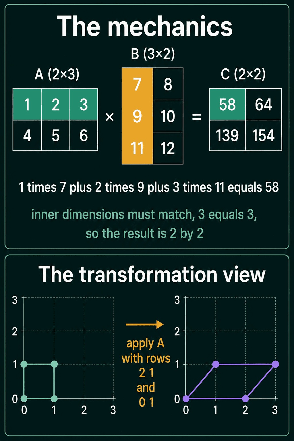
Two things trip people up early. The shapes have to line up, so a $3 \times 4$ matrix cannot multiply a $2 \times 5$ matrix. The order also changes the result: $AB$ and $BA$ are usually different matrices, and one of them may not even be defined. With the $A$ and $B$ above, $AB$ is $2 \times 2$ and $BA$ is $3 \times 3$. Matrix multiplication is not commutative.
The transformation view: a matrix is a function
The row-times-column rule says how to compute a product. What the product means is clearer when a matrix multiplies a single vector. $A\mathbf{x}$ takes a vector $\mathbf{x}$ in and returns a new vector out, stretched, rotated, squashed, or some mix of those. Read this way, a matrix is a function on vectors, often called a linear map. Multiplying a matrix by a whole stack of vectors applies that same function to every one of them at once.
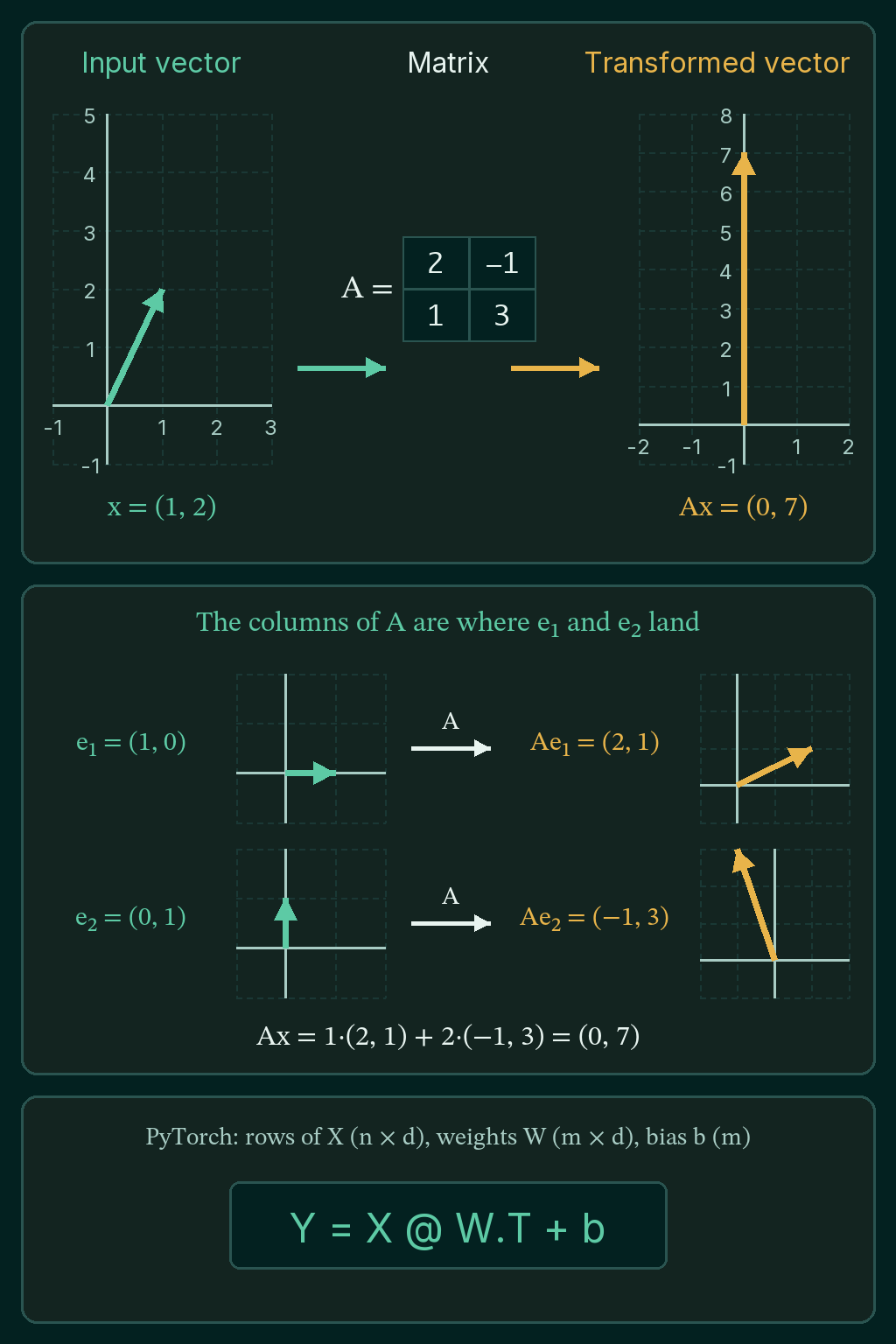
The columns of $A$ say exactly what the function does. Write $\mathbf{e}_1 = (1, 0, 0, \ldots)$ for the vector with a 1 in the first position and zeros elsewhere, $\mathbf{e}_2 = (0, 1, 0, \ldots)$ for the second position, and so on. These are the standard basis vectors. Computing $A\mathbf{e}_j$, every term drops out except the one that meets the 1, which leaves column $j$ of $A$. Every other vector is a sum of scaled basis vectors, so knowing where the basis vectors land tells you where everything lands.
The bottom of the picture above shows this for the matrix with rows $(2, 1)$ and $(0, 1)$. Its first column is $(2, 0)$, so the corner of the square at $(1, 0)$ moves to $(2, 0)$. Its second column is $(1, 1)$, so the corner at $(0, 1)$ moves to $(1, 1)$, and the square becomes a slanted parallelogram.
Take $A$ with rows $(2, -1)$ and $(1, 3)$. Its columns are $(2, 1)$ and $(-1, 3)$, so $A\mathbf{e}_1 = (2, 1)$ and $A\mathbf{e}_2 = (-1, 3)$. The vector $\mathbf{x} = (1, 2)$ is $1 \cdot \mathbf{e}_1 + 2 \cdot \mathbf{e}_2$, so $A\mathbf{x}$ is $1 \cdot (2, 1) + 2 \cdot (-1, 3) = (0, 7)$.
This is the working model behind most neural network layers. nn.Linear(in_features, out_features) holds a matrix that maps a vector with in_features entries to one with out_features entries. One PyTorch detail: the stored weight has shape (out_features, in_features), and the layer computes x @ W.T + b, where x holds one input vector per row, W.T is the transpose of the stored weight (its rows and columns swapped), and b is the added bias vector.
Outer products: the other way to multiply two vectors
A dot product needs two vectors of the same length and collapses them into one number. The outer product has no length requirement. For $\mathbf{x}$ with $m$ entries and $\mathbf{y}$ with $n$ entries, the outer product $\mathbf{x}\mathbf{y}^T$ is an $m \times n$ matrix whose entry in row $i$ and column $j$ is $x_i y_j$. Here $\mathbf{x}$ is treated as an $m \times 1$ column and $\mathbf{y}^T$ as a $1 \times n$ row, and multiplying them with the usual rule gives the $m \times n$ result.
With $\mathbf{x} = (1, 2, 3)$ and $\mathbf{y} = (4, 5)$, a $3 \times 1$ times a $1 \times 2$ gives a $3 \times 2$ matrix:
$$\mathbf{x}\mathbf{y}^T = \begin{bmatrix} 4 & 5 \ 8 & 10 \ 12 & 15 \end{bmatrix}$$
Each row of the result is $\mathbf{y}$ scaled by one entry of $\mathbf{x}$.
Matrix multiplication as a sum of outer products
Outer products give a second way to build the whole product $AB$ at once instead of entry by entry. Pair column $k$ of $A$, called $\mathbf{a}_k$, with row $k$ of $B$, called $\mathbf{b}_k^T$. Each pair gives an outer product the same shape as $AB$, and adding all of them gives $AB$:
$$AB = \sum_{k=1}^{p} \mathbf{a}_k \mathbf{b}_k^T$$
This gives exactly the same matrix as the row-times-column formula.
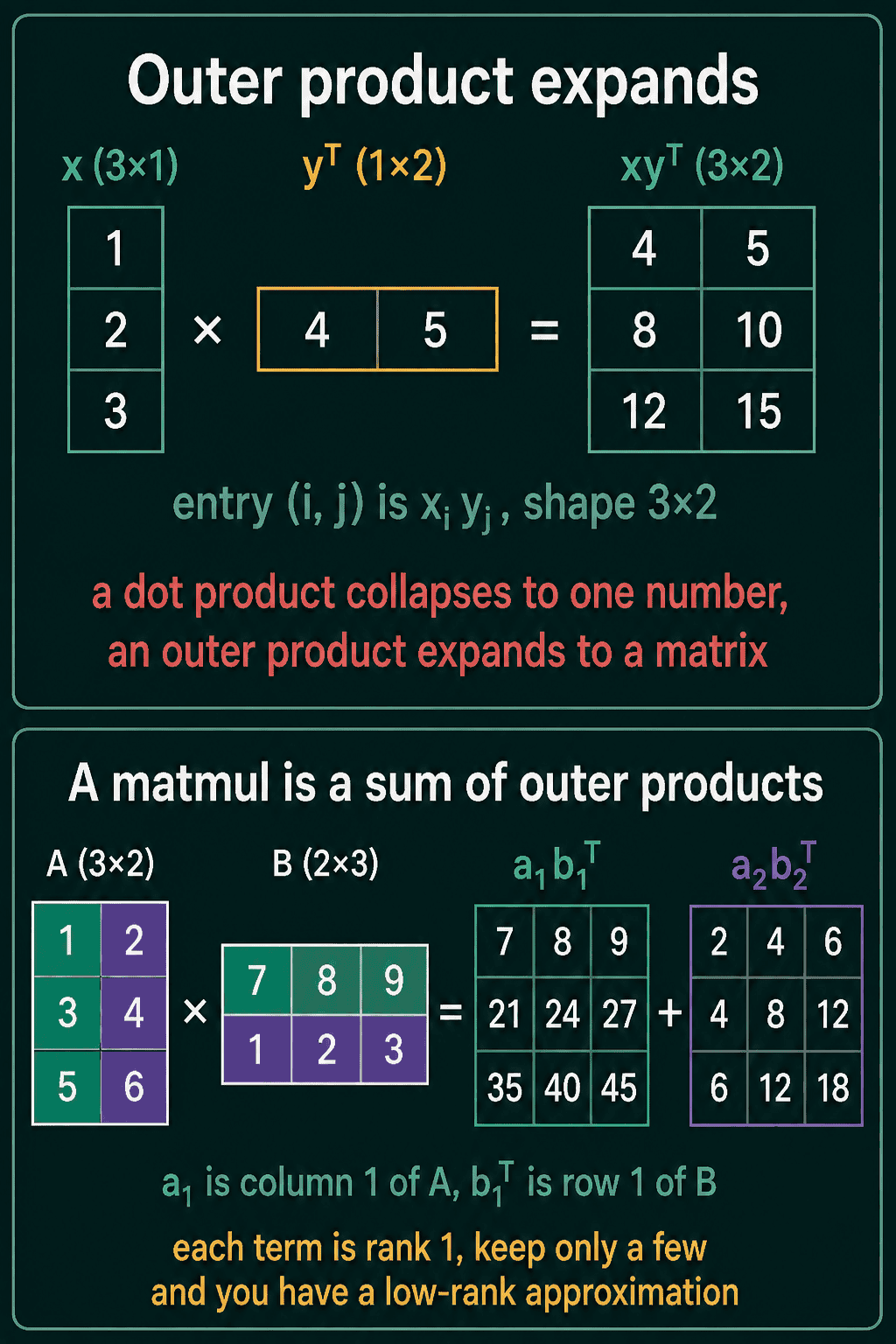
Each outer product is built from a single direction, which makes it a rank 1 matrix, the simplest kind there is (as long as neither vector is all zeros). Keeping only a few of the terms in the sum, instead of all $p$, gives a matrix close to $AB$ built from a few directions, which is the idea behind a low-rank approximation.
A matrix times a vector also has two readings. Row by row, entry $i$ of $A\mathbf{x}$ is the dot product of row $i$ of $A$ with $\mathbf{x}$. Column by column, $A\mathbf{x}$ is a sum of the columns of $A$, each scaled by the matching entry of $\mathbf{x}$. Both give the same vector, and switching between them is often the fastest way to see why a matrix operation does what it does.
Matrix multiplication in PyTorch
@ and torch.matmul both do matrix multiplication. The code below checks the claims in this post on the same numbers.
1import torch
2
3A = torch.tensor([[1., 2., 3.],
4                  [4., 5., 6.]])        # shape (2, 3)
5B = torch.tensor([[7., 8.],
6                  [9., 10.],
7                  [11., 12.]])          # shape (3, 2)
8
9C = A @ B
10print(C, C.shape)
11print(torch.dot(A[0], B[:, 0]))         # row 1 of A dotted with column 1 of B
12
13# B @ A is also defined, and it is a different matrix with a different shape
14print((B @ A).shape)
15
16# the columns of a matrix are where the basis vectors land
17M = torch.tensor([[2., 1.],
18                  [0., 1.]])
19print(M @ torch.tensor([1., 0.]), M @ torch.tensor([0., 1.]))
20
21# outer product: (3,) and (2,) give a (3, 2) matrix
22x = torch.tensor([1., 2., 3.])
23y = torch.tensor([4., 5.])
24print(torch.outer(x, y))
25
26# a matmul is a sum of outer products, one per column of P and row of Q
27P = torch.tensor([[1., 2.], [3., 4.], [5., 6.]])
28Q = torch.tensor([[7., 8., 9.], [1., 2., 3.]])
29total = torch.outer(P[:, 0], Q[0]) + torch.outer(P[:, 1], Q[1])
30print(torch.equal(total, P @ Q))
31
32# nn.Linear stores its weight as (out_features, in_features) and computes x @ W.T + b
33layer = torch.nn.Linear(3, 2)
34inp = torch.randn(4, 3)                 # a batch of 4 vectors with 3 features each
35print(layer.weight.shape, layer(inp).shape)
36print(torch.allclose(layer(inp), inp @ layer.weight.T + layer.bias))1tensor([[ 58., 64.],
2 [139., 154.]]) torch.Size([2, 2])
3tensor(58.)
4torch.Size([3, 3])
5tensor([2., 0.]) tensor([1., 1.])
6tensor([[ 4., 5.],
7 [ 8., 10.],
8 [12., 15.]])
9True
10torch.Size([2, 3]) torch.Size([4, 2])
11TrueWhen a matrix multiplication fails with a shape error, print the .shape of both sides first and check that the last dimension of the left one equals the first dimension of the right one.
Common mistakes
- Mismatched inner dimensions. $(3, 4)$ times $(4, 5)$ works and gives $(3, 5)$, while $(3, 4)$ times $(5, 4)$ fails, and transposing one side is often the fix.
- Swapping the order. $AB$ and $BA$ are usually different, so
B @ Ain place ofA @ Bgives a wrong result or a shape error. - Forgetting the transpose in
nn.Linear. The stored weight is(out_features, in_features), so computing a layer by hand needsx @ W.T, notx @ W. - Using
*for matrix multiplication. In PyTorch*multiplies matching positions and@multiplies rows by columns, and on two square matrices both run without an error.
Related math
The Hadamard product is the position-by-position product that * computes, compared side by side with @ in Hadamard product vs matrix multiplication. Vectors, matrices and the transpose are covered in vectors and matrices for machine learning.
QuiddityML teaches matrix multiplication and outer products as two concepts in the linear algebra part of the Math track, and the exercises include tracing shapes through a two-layer transformation, spotting the bug in a hand-written linear layer, and writing outer_product without torch.outer.