By Sagi Shaier · 12 October 2026 · 9 min read
Matrix calculus for deep learning: the gradient of a linear layer, by hand
A gentle walk through the few vector and matrix gradients deep learning reuses, with small examples you can check by hand, ending with the backward pass of a linear layer worked out with real numbers and checked in PyTorch.
Matrix calculus is ordinary calculus applied to expressions made of vectors and matrices. Training a neural network means asking, for every weight, how much the loss would change if that weight moved a little. Most layers are built from vectors and matrices, so those answers come from a handful of matrix-calculus rules, and the most used one is the rule for a linear layer.
Vectors, matrices, and the transpose
A vector is a list of numbers, such as $x = [2, 5]$. A matrix is a grid of numbers with rows and columns. This one has 2 rows and 3 columns, so its shape is $2 \times 3$:
$$A = \begin{bmatrix} 1 & 2 & 3 \\ 4 & 5 & 6 \end{bmatrix}$$
The transpose of a matrix, written $A^T$, swaps its rows and columns. The first row of $A$ becomes the first column of $A^T$, and the second row becomes the second column:
$$A^T = \begin{bmatrix} 1 & 4 \\ 2 & 5 \\ 3 & 6 \end{bmatrix}$$
$A$ was $2 \times 3$, so $A^T$ is $3 \times 2$. Most formulas below use a transpose.
Multiplying two vectors entry by entry and adding the results is called a dot product. For $a = [3, 4]$ and $x = [2, 5]$ it is $3 \cdot 2 + 4 \cdot 5 = 26$. In matrix notation it is written $a^T x$.
What a gradient is
Take a function that turns a vector into one number, such as $f(x) = 3x_1 + 4x_2$. At $x = [2, 5]$ it gives $3 \cdot 2 + 4 \cdot 5 = 26$.
Now nudge one input and watch the output. If $x_1$ goes from 2 to 2.01, the output goes from 26 to 26.03. It moved 3 times as much as the input did, so the slope of $f$ along $x_1$ is 3. That slope, measured along one input while the others stay put, is called a partial derivative and written $\frac{\partial f}{\partial x_1}$. Doing the same for $x_2$ gives a slope of 4.
The gradient collects one partial derivative per input into a vector. For this $f$ the gradient is $[3, 4]$, written $\nabla_x f = [3, 4]$. The symbol $\nabla_x$ reads as "the gradient with respect to $x$".
Gradients worth knowing by sight
The same few expressions come up again and again in ML derivations. Each one below can be worked out one partial derivative at a time, and each gives a short answer worth recognizing on sight.
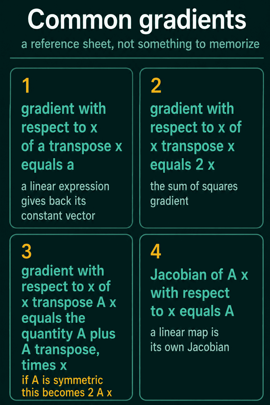
A dot product with a constant vector. The function above was $f(x) = a^T x$ with $a = [3, 4]$, and its gradient came out as $[3, 4]$, which is $a$ itself. That holds for any constant vector $a$:
$$\nabla_x (a^T x) = a$$
A sum of squares. $x^T x$ is the dot product of $x$ with itself, so for $x = [2, 5]$ it is $2^2 + 5^2 = 29$. The slope of $x_1^2$ along $x_1$ is $2x_1 = 4$, and the slope of $x_2^2$ along $x_2$ is $2x_2 = 10$. The gradient is $[4, 10]$, which is $2x$:
$$\nabla_x (x^T x) = 2x$$
A quadratic form. $x^T A x$ multiplies $x$ by a square matrix $A$ and then takes the dot product with $x$ again. Its gradient is
$$\nabla_x (x^T A x) = (A + A^T)x$$
When $A$ equals its own transpose, which is called a symmetric matrix, $A + A^T$ is $2A$ and the gradient becomes $2Ax$. For $A = \begin{bmatrix} 2 & 1 \\ 1 & 3 \end{bmatrix}$ and $x = [1, 2]$, that gives $2Ax = 2 \cdot [4, 7] = [8, 14]$.
A matrix times a vector. $Ax$ turns one vector into another, so its derivative is a matrix called the Jacobian: one row per output and one column per input, each entry the slope of one output along one input. For $Ax$ that matrix is $A$ itself. With $A = \begin{bmatrix} 1 & 2 \\ 0 & 3 \end{bmatrix}$, the outputs are $x_1 + 2x_2$ and $3x_2$. Their slopes along $x_1$ and $x_2$ are $[1, 2]$ and $[0, 3]$, which are the rows of $A$.
A squared-error loss. A linear model with inputs $A$, weights $x$ and targets $b$ has errors $Ax - b$, and the sum of their squares $\|Ax - b\|^2$ is the loss. Its gradient is
$$\nabla_x \|Ax - b\|^2 = 2A^T(Ax - b)$$
The $2(Ax - b)$ part comes from the sum-of-squares rule applied to the errors. The $A^T$ in front comes from the chain rule, which multiplies by the derivative of the inner expression $Ax - b$.
The shape rule
A gradient has the same shape as the thing it is taken with respect to. In the examples above, $x$ had 2 entries and every gradient with respect to $x$ had 2 entries. For a weight matrix of shape $3 \times 2$, the gradient with respect to it is also $3 \times 2$. If a hand-derived gradient comes out with any other shape, the derivation went wrong somewhere, and this check usually catches the error before the algebra is done.
A linear layer with real numbers
A linear layer multiplies its input by a weight matrix: $y = xw$. Take one input row with 3 numbers and a weight matrix with 3 rows and 2 columns:
$$x = \begin{bmatrix} 1 & 2 & 3 \end{bmatrix} \qquad w = \begin{bmatrix} 1 & 0 \\ 0 & 1 \\ 1 & 1 \end{bmatrix}$$
Each output is a dot product of $x$ with one column of $w$. The first column gives $y_1 = 1 \cdot 1 + 2 \cdot 0 + 3 \cdot 1 = 4$, and the second gives $y_2 = 1 \cdot 0 + 2 \cdot 1 + 3 \cdot 1 = 5$. So $y = [4, 5]$.
During training, the layers after this one turn $y$ into a loss $L$. Backpropagation works from the loss backward, so by the time it reaches this layer it already has $\frac{\partial L}{\partial y}$: how much the loss changes per unit change in each output. Say it is $[1, 2]$. That means nudging $y_1$ up by a small amount raises the loss by 1 times that amount, and nudging $y_2$ raises it by 2 times.
The layer has to answer two questions. How does the loss change with each input, $\frac{\partial L}{\partial x}$, so the layer before it can keep going backward? And how does the loss change with each weight, $\frac{\partial L}{\partial w}$, so these weights can be updated?
The gradient for each input
Follow $x_1$ through the layer. It reaches $y_1$ through the weight $w_{11} = 1$ and reaches $y_2$ through $w_{12} = 0$. Nudging $x_1$ by a small amount therefore moves $y_1$ by 1 times that amount and $y_2$ by 0 times. Each of those output changes moves the loss by its own entry of $\frac{\partial L}{\partial y}$, and the effects add up:
$$\frac{\partial L}{\partial x_1} = 1 \cdot 1 + 2 \cdot 0 = 1$$
The same walk for $x_2$ uses its weights $w_{21} = 0$ and $w_{22} = 1$, and for $x_3$ it uses $w_{31} = 1$ and $w_{32} = 1$:
$$\frac{\partial L}{\partial x_2} = 1 \cdot 0 + 2 \cdot 1 = 2 \qquad \frac{\partial L}{\partial x_3} = 1 \cdot 1 + 2 \cdot 1 = 3$$
So $\frac{\partial L}{\partial x} = [1, 2, 3]$. Each entry was the dot product of $\frac{\partial L}{\partial y}$ with one row of $w$. Taking dot products with the rows of $w$ is the same as multiplying by $w^T$, whose columns are those rows:
$$\frac{\partial L}{\partial x} = \frac{\partial L}{\partial y}\, w^T$$
The gradient for each weight
A single weight $w_{ij}$ connects input $x_i$ to output $y_j$ and touches nothing else. Nudging it moves $y_j$ by $x_i$ times the nudge, and that moves the loss by $\frac{\partial L}{\partial y_j}$ times as much. So each weight's gradient is a plain product:
$$\frac{\partial L}{\partial w_{ij}} = x_i \cdot \frac{\partial L}{\partial y_j}$$
With $x = [1, 2, 3]$ and $\frac{\partial L}{\partial y} = [1, 2]$, row $i$ of the result is $x_i$ times $[1, 2]$:
$$\frac{\partial L}{\partial w} = \begin{bmatrix} 1 & 2 \\ 2 & 4 \\ 3 & 6 \end{bmatrix}$$
That grid is $x^T$, the input turned into a column, multiplied by the row $\frac{\partial L}{\partial y}$:
$$\frac{\partial L}{\partial w} = x^T \frac{\partial L}{\partial y}$$
The shape rule agrees. $w$ is $3 \times 2$ and so is its gradient. $x$ has 3 entries and so does its gradient.
The same formulas for a whole batch
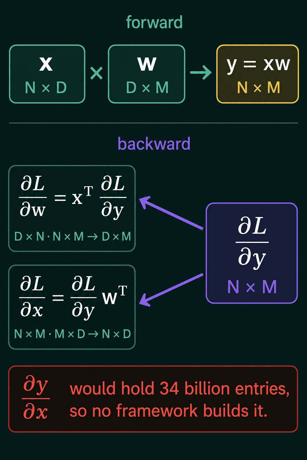
Real layers process many input rows at once. Stack $N$ input rows of $D$ numbers each into an $N \times D$ matrix $x$, and use a $D \times M$ weight matrix $w$. The output $y = xw$ is $N \times M$, one row of outputs per input row. The two formulas stay exactly the same:
$$\frac{\partial L}{\partial x} = \frac{\partial L}{\partial y}\, w^T \qquad \frac{\partial L}{\partial w} = x^T \frac{\partial L}{\partial y}$$
The shapes still line up. $\frac{\partial L}{\partial y}$ is $N \times M$ and $w^T$ is $M \times D$, giving $N \times D$ like $x$. $x^T$ is $D \times N$ and $\frac{\partial L}{\partial y}$ is $N \times M$, giving $D \times M$ like $w$.
Why frameworks use these formulas instead of the Jacobian
The general chain rule would build the Jacobian of $y$ with respect to $x$: one row for every entry of $y$ and one column for every entry of $x$. For a realistic layer with $N = 128$, $D = 1024$ and $M = 2048$, that matrix has $(128 \cdot 2048) \times (128 \cdot 1024)$ entries. That is over 34 billion numbers, about 137 GB in 32-bit floats. The two short formulas above give the same gradients without ever building it, using one matrix multiplication each.
Checking it in PyTorch
PyTorch's autograd computes these gradients when .backward() runs and stores them in x.grad and w.grad. Choosing the loss $L = 1 \cdot y_1 + 2 \cdot y_2$ makes $\frac{\partial L}{\partial y} = [1, 2]$, so the result should match the hand calculation.
1import torch
2
3x = torch.tensor([[1.0, 2.0, 3.0]], requires_grad=True)
4w = torch.tensor([[1.0, 0.0],
5                  [0.0, 1.0],
6                  [1.0, 1.0]], requires_grad=True)
7
8y = x @ w
9print(y)          # tensor([[4., 5.]])
10
11L = (y * torch.tensor([[1.0, 2.0]])).sum()   # dL/dy = [1, 2]
12L.backward()
13print(x.grad)     # tensor([[1., 2., 3.]])
14print(w.grad)     # tensor([[1., 2.], [2., 4.], [3., 6.]])
The same check works on random batches, where the formulas are compared with autograd instead of with hand-computed numbers:
1import torch
2
3torch.manual_seed(0)
4N, D, M = 4, 3, 2
5x = torch.randn(N, D, requires_grad=True)
6w = torch.randn(D, M, requires_grad=True)
7
8y = x @ w
9L = (y ** 2).sum()      # here dL/dy = 2y
10L.backward()
11
12dL_dy = 2 * y.detach()
13print(torch.allclose(x.grad, dL_dy @ w.detach().T))   # True
14print(torch.allclose(w.grad, x.detach().T @ dL_dy))   # True
If a hand-written backward pass fails a check like this, compare the shapes first. A missing transpose usually shows up as a gradient with the shape of the wrong variable.
Common mistakes
- Missing transpose. $\frac{\partial L}{\partial y}\, w$ instead of $\frac{\partial L}{\partial y}\, w^T$ gives the wrong numbers, and usually the wrong shape.
- Wrong multiplication order. The weight gradient is $x^T \frac{\partial L}{\partial y}$, with $x^T$ on the left. The reversed order does not have matching inner dimensions.
- Using $2Ax$ for a matrix that is not symmetric. For a general $A$ the gradient of $x^T A x$ is $(A + A^T)x$.
- Dropping the 2. The gradients of $x^T x$ and $\|Ax - b\|^2$ both carry a 2 from the square.
Related concepts
Partial derivatives and gradients are the slopes this post builds on, one input at a time. The chain rule is what adds up the effect of each input through every output it touches, which is the sum in the input-gradient walk above. The Jacobian matrix is the derivative of a vector-to-vector function, and the linear-layer formulas are the chain rule with that Jacobian never written out. Automatic differentiation stores a backward formula like these for each operation and applies them in reverse order when .backward() runs.
QuiddityML teaches matrix calculus and backpropagation through a linear layer as two concepts in the Math track, and the exercises include filling in the transpose formulas for y = x @ w and writing linear_backward from scratch.