By Sagi Shaier · 12 October 2026 · 5 min read

The Jacobian matrix explained

How to build the Jacobian of a function with several inputs and outputs, why the gradient is a one-row Jacobian, and how to use it to chain layers and estimate output sensitivity, with PyTorch checks.

The Jacobian is the matrix of every partial derivative of a function that takes a vector in and returns a vector out: one row per output, one column per input. Most layers in a neural network are functions of that kind, so the Jacobian is what describes how a layer's outputs respond when its inputs move, and the chain rule for networks is written as a product of Jacobians.

Why a single slope is not enough

For a function with one input and one output, the derivative is one number: the slope. For a function with many inputs and one output, such as a loss, the derivative is the gradient. The gradient is a vector holding one partial derivative per input. A partial derivative is the slope with respect to one input while every other input is held fixed.

A linear layer does not fit either case. It takes a vector of numbers in and returns a different vector of numbers. Each output can change with each input, so there is one slope for every pair of output and input, and those slopes need a matrix to hold them.

The definition

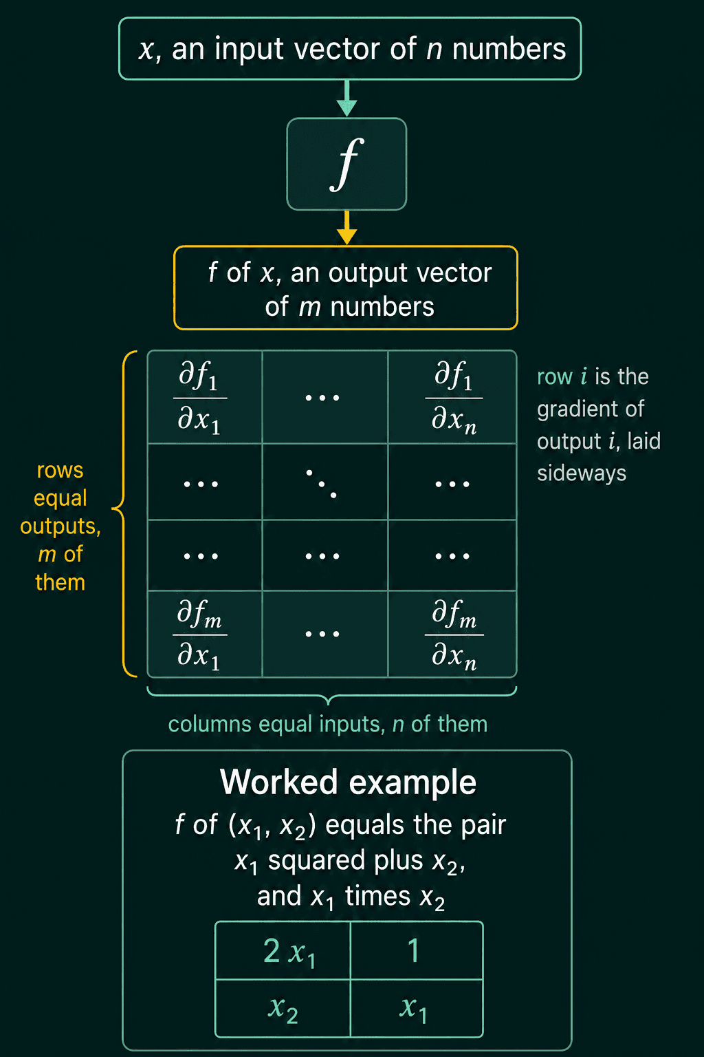
Let $f$ take an input vector $x$ with $n$ entries and return an output vector with $m$ entries, $f_1$ through $f_m$. The Jacobian $J$ is the $m \times n$ matrix whose entry in row $i$ and column $j$ is the partial derivative of output $i$ with respect to input $j$:

$$J = \begin{bmatrix} \frac{\partial f_1}{\partial x_1} & \cdots & \frac{\partial f_1}{\partial x_n} \\ \vdots & \ddots & \vdots \\ \frac{\partial f_m}{\partial x_1} & \cdots & \frac{\partial f_m}{\partial x_n} \end{bmatrix}$$

Reading across row $i$ gives the slopes of output $f_i$ with respect to every input. That row is the gradient of $f_i$, laid on its side as $\nabla f_i(x)^T$.

The gradient is a one-row Jacobian

When the function has a single output ($m = 1$), the Jacobian has a single row: a $1 \times n$ matrix whose entries are the partial derivatives of that one output. That row holds the same numbers as the gradient. The gradient and the Jacobian are one idea, and the gradient is the case with one output.

A worked example

Take a function with 2 inputs and 2 outputs:

$$f(x_1, x_2) = \big[x_1^2 + x_2,\ x_1 x_2\big]$$

Call the outputs $f_1 = x_1^2 + x_2$ and $f_2 = x_1 x_2$. Row 1 holds the partial derivatives of $f_1$: $\frac{\partial f_1}{\partial x_1} = 2x_1$ and $\frac{\partial f_1}{\partial x_2} = 1$. Row 2 holds the partial derivatives of $f_2$: $\frac{\partial f_2}{\partial x_1} = x_2$ and $\frac{\partial f_2}{\partial x_2} = x_1$.

$$J = \begin{bmatrix} 2x_1 & 1 \\ x_2 & x_1 \end{bmatrix}$$

Each entry is an ordinary partial derivative. The Jacobian adds the bookkeeping: one row per output, one column per input. At the point $x = (3, 2)$ it is

$$J = \begin{bmatrix} 6 & 1 \\ 2 & 3 \end{bmatrix}$$

An input vector x of n numbers goes into f and comes out as f of x, an output vector of m numbers, above the m by n grid of partial derivatives with rows labelled as outputs and columns as inputs, row i described as the gradient of output i laid sideways, and a worked example box with the Jacobian 2 x1, 1, x2, x1 for f of x1, x2 equal to x1 squared plus x2 and x1 times x2

Estimating how much an output moves

If an input shifts by a small amount $\Delta x$, from measurement noise or rounding for example, the Jacobian estimates the resulting shift in the output $\Delta y$ without rerunning the function:

$$\Delta y \approx J\, \Delta x$$

The estimate is good only for small shifts. $J$ also depends on where it is evaluated, so it has to be recomputed at each new input. In the example above at $x = (3, 2)$, a shift of $\Delta x = (0.01, -0.02)$ gives

$$J\,\Delta x = (6 \cdot 0.01 - 0.02,\ 2 \cdot 0.01 - 3 \cdot 0.02) = (0.04,\ -0.04)$$

Running the function at the shifted point gives a true change of $(0.0401, -0.0402)$, so the linear estimate is off only in the fourth decimal place.

Chaining layers: the Jacobian in the chain rule

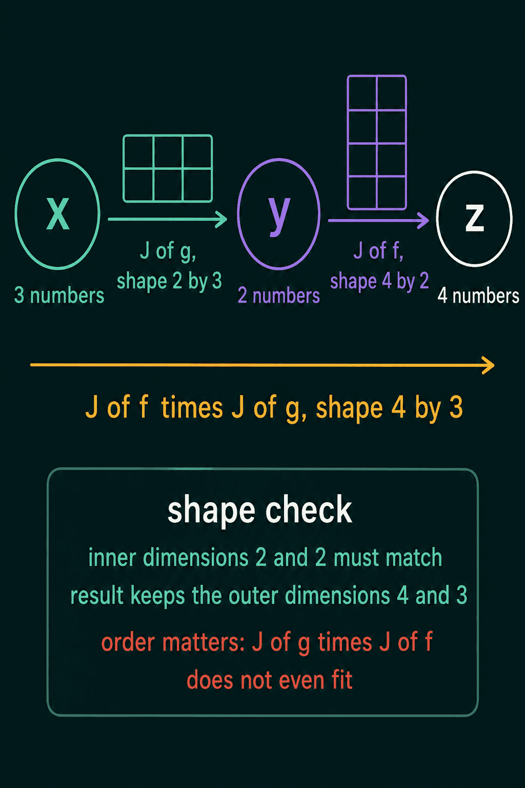
When $y = g(x)$ feeds $z = f(y)$, the Jacobian of the whole composition is the product of the two Jacobians, outer on the left:

$$J_{f \circ g}(x) = J_f(y) \cdot J_g(x)$$

Here $f \circ g$ means "apply $g$, then $f$", and $J_f(y)$ is evaluated at $y = g(x)$. Shapes give a quick check on the order. A $g$ from 3 numbers to 2 has a $2 \times 3$ Jacobian, and an $f$ from 2 numbers to 4 has a $4 \times 2$ one. Their product $J_f \cdot J_g$ is $4 \times 3$, which is the right shape for 3 inputs and 4 outputs. The reversed product does not have matching inner dimensions.

x with 3 numbers maps through J of g, shape 2 by 3, to y with 2 numbers, then through J of f, shape 4 by 2, to z with 4 numbers, with J of f times J of g giving shape 4 by 3 and a shape check box noting that the inner dimensions 2 and 2 must match and that J of g times J of f does not fit

Computing a Jacobian in PyTorch

torch.autograd.functional.jacobian takes a function and a point and returns the full Jacobian there.

1import torch
2from torch.autograd.functional import jacobian
3 
4def f(x):
5    return torch.stack([x[0] ** 2 + x[1], x[0] * x[1]])
6 
7x = torch.tensor([3.0, 2.0])
8J = jacobian(f, x)
9print(J)
10# tensor([[6., 1.],
11#         [2., 3.]])
12 
13dx = torch.tensor([0.01, -0.02])
14print(J @ dx)              # tensor([ 0.0400, -0.0400]), the estimate
15print(f(x + dx) - f(x))    # tensor([ 0.0401, -0.0402]), the true change

If the shape comes back transposed from what you expected, check the convention first: rows are outputs and columns are inputs, so a function from 3 numbers to 4 has a $4 \times 3$ Jacobian.

When to use it, and common mistakes

Build the full Jacobian when you want to study a small function: to check a hand derivation, or to see which input an output is most sensitive to. For the large layers inside a real network, frameworks skip building it. A linear layer with a batch of 128 inputs of size 1024 and 2048 outputs would have a Jacobian with over 34 billion entries, so backpropagation uses direct formulas that give the same gradients without forming that matrix.

Rows and columns swapped. The Jacobian is (outputs) $\times$ (inputs). A function from $\mathbb{R}^3$ to $\mathbb{R}^4$ has a $4 \times 3$ Jacobian, not $3 \times 4$.
Treating it as a constant. Outside linear functions, the Jacobian changes from point to point. The example above is $\begin{bmatrix} 6 & 1 \\ 2 & 3 \end{bmatrix}$ only at $x = (3, 2)$.
Using $J\,\Delta x$ for large shifts. The estimate is a linear approximation, and it drifts from the true change as $\Delta x$ grows.

Partial derivatives and gradients are the entries of the Jacobian and the single-output case of it. The chain rule for vector functions is a product of Jacobians. Matrix calculus collects ready-made gradients and Jacobians for common expressions: the Jacobian of $Ax$ with respect to $x$ is $A$ itself, because $Ax$ is a linear map. Backpropagation through a linear layer uses that structure to get gradients without ever building the full Jacobian.

QuiddityML teaches the Jacobian as its own concept in the Math track, and the exercises on it include filling in the entries for a two-output function and writing a jacobian function from scratch in PyTorch.