By Sagi Shaier · 12 October 2026 · 6 min read

The chain rule explained for machine learning

How to differentiate a function that feeds into another function, how the rule extends to several paths and to vector-valued layers, and how to check the result in PyTorch.

The chain rule is the rule for differentiating a function whose input is the output of another function: take the derivative of the outer function, take the derivative of the inner function, and multiply them. A neural network passes each layer's output into the next layer, so its loss is one long chain of functions, and the chain rule is how each weight in that chain gets its own gradient during training.

The problem: a function whose input is another function's output

The basic derivative rules, such as the power rule and the product rule, work when a function's input is the variable you are differentiating with respect to. Take $z = (3x+1)^2$. The squaring does not act on $x$ directly. It acts on $3x+1$, which itself depends on $x$.

A function built this way is called a composition. Write the inner part as $y = g(x)$ and the outer part as $z = f(y)$. Then $z$ depends on $x$ only through $y$, and neither $f'$ nor $g'$ on its own gives $\frac{dz}{dx}$, because $x$ is not $f$'s direct input.

The rule for one input

Differentiate the outer function with respect to its own input $y$ and the inner function with respect to $x$, then multiply the two:

$$\frac{dz}{dx} = \frac{dz}{dy} \cdot \frac{dy}{dx}$$

Here $\frac{dz}{dy}$ is how fast $z$ changes when $y$ moves, and $\frac{dy}{dx}$ is how fast $y$ changes when $x$ moves. Their product is how fast $z$ changes when $x$ moves.

For $z = (3x+1)^2$, the inner function is $y = 3x+1$ and the outer function is $z = y^2$:

$$\frac{dz}{dy} = 2y \qquad \frac{dy}{dx} = 3$$

$$\frac{dz}{dx} = 2y \cdot 3 = 6(3x+1)$$

At $x = 2$ this gives $6 \cdot 7 = 42$.

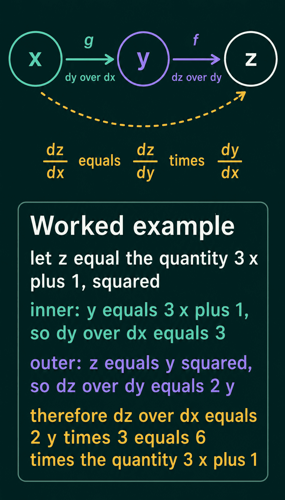
The chain x to y to z, with dy over dx labelling the arrow from x to y and dz over dy labelling the arrow from y to z, the product rule dz over dx equals dz over dy times dy over dx, and a worked example box for z equal to 3x plus 1 squared ending at 6 times the quantity 3x plus 1

Longer chains work the same way. If $x$ feeds $y$ and $y$ feeds $u$ and $u$ feeds $z$, then $\frac{dz}{dx}$ is the product of the three local derivatives.

When a variable reaches the output by more than one path

In a network, one number often feeds several later quantities. Say $x$ feeds two intermediates, $y_1 = x^2$ and $y_2 = 3x$, and the output combines them as $z = y_1 y_2$. There are now two routes from $x$ to $z$.

Each route contributes the product of its own local derivatives, and the contributions add:

$$\frac{dz}{dx} = \frac{\partial z}{\partial y_1}\frac{dy_1}{dx} + \frac{\partial z}{\partial y_2}\frac{dy_2}{dx}$$

The curly $\partial$ marks a partial derivative: the derivative with respect to one input while the other inputs are held fixed. Here $\frac{\partial z}{\partial y_1} = y_2$ and $\frac{\partial z}{\partial y_2} = y_1$, so

$$\frac{dz}{dx} = 3x \cdot 2x + x^2 \cdot 3 = 9x^2$$

At $x = 2$ that is 36. The general form, for an output $z_k$ that depends on $x_i$ through intermediates $y_1, \ldots, y_m$, is a sum over every intermediate:

$$\frac{\partial z_k}{\partial x_i} = \sum_j \frac{\partial z_k}{\partial y_j}\frac{\partial y_j}{\partial x_i}$$

This sum over paths is the form backpropagation uses. A loss is a single number, so in that case there is only one output and the index $k$ drops away.

The chain rule for vector-valued layers

A linear layer takes a vector in and returns a different vector. An activation function then maps that vector to another vector of the same size. So the functions a network composes are vector-to-vector, and each derivative in the chain becomes a matrix.

That matrix is the Jacobian. For a function with $n$ inputs and $m$ outputs, the Jacobian is an $m \times n$ matrix with one row per output and one column per input, and each entry is the partial derivative of one output with respect to one input. Write $J_g(x)$ for the Jacobian of $g$ at the point $x$.

If $y = g(x)$ and $z = f(y)$ for vectors $x$, $y$ and $z$ of possibly different sizes, the chain rule becomes a matrix product:

$$J_{f \circ g}(x) = J_f(y) \cdot J_g(x)$$

The symbol $f \circ g$ means "apply $g$, then $f$". The equation says the Jacobian of the composition is the outer Jacobian at $y = g(x)$ times the inner Jacobian at $x$. Each entry of that product is exactly the sum over paths from the previous section.

The order of the two Jacobians is fixed because matrix multiplication is not commutative. Only one order has matching inner dimensions. If $g$ takes 3 numbers to 2, then $J_g$ is $2 \times 3$. If $f$ takes those 2 numbers to 4, then $J_f$ is $4 \times 2$. The product $J_f \cdot J_g$ is $4 \times 3$, which is the right shape for a function with 3 inputs and 4 outputs. The other order $J_g \cdot J_f$ multiplies a $2 \times 3$ by a $4 \times 2$, and those inner dimensions (3 and 4) do not match.

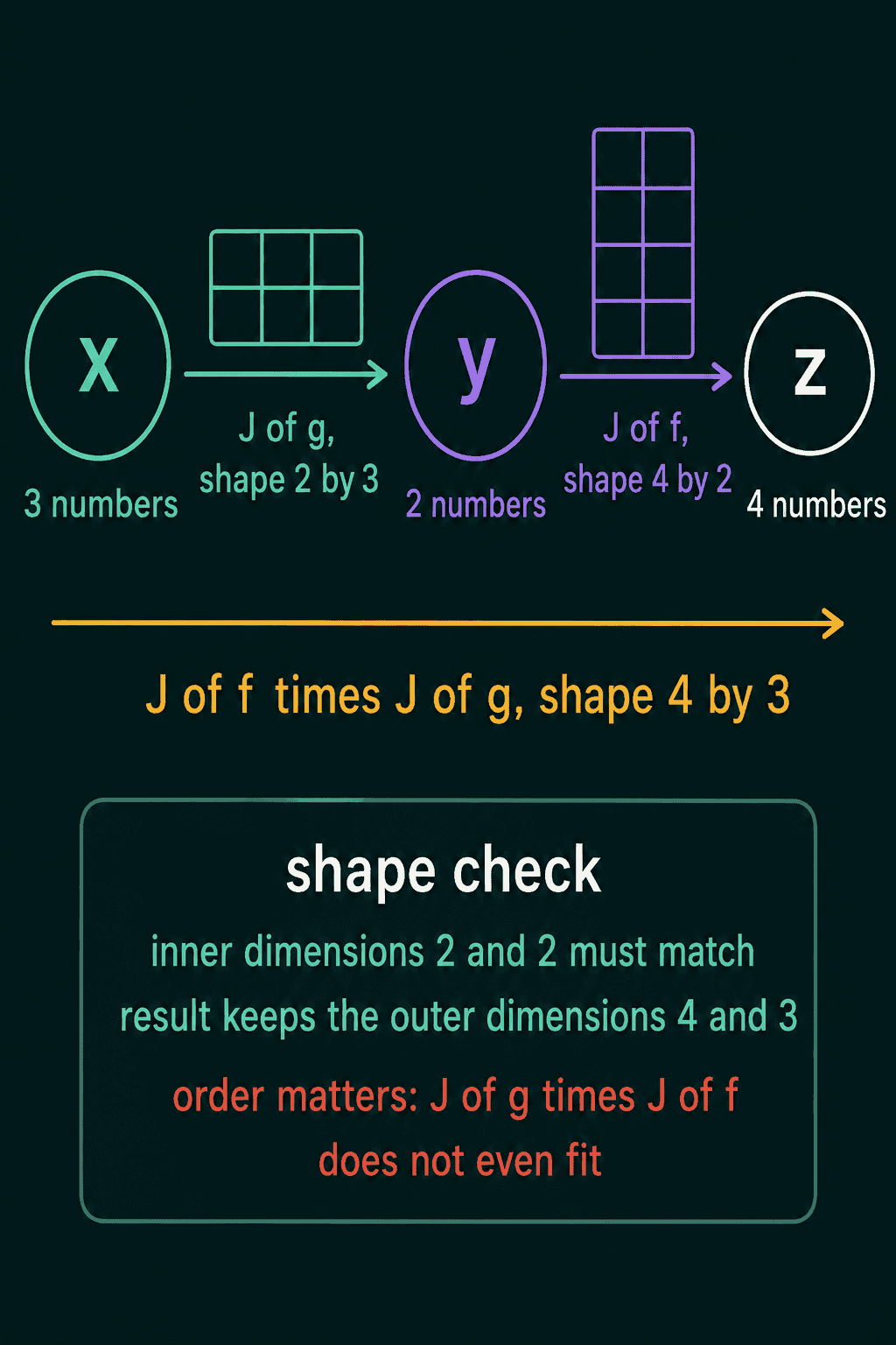
x with 3 numbers maps through J of g, shape 2 by 3, to y with 2 numbers, then through J of f, shape 4 by 2, to z with 4 numbers, with J of f times J of g giving shape 4 by 3 and a shape check box noting that the inner dimensions 2 and 2 must match and that J of g times J of f does not fit

The single-input rule above is the same equation with every Jacobian of size $1 \times 1$.

Checking the chain rule in PyTorch

PyTorch's autograd records each operation as it runs and applies the chain rule backward through them when you call .backward(). The derivative it stores in x.grad should match the hand calculation.

1import torch
2 
3x = torch.tensor(2.0, requires_grad=True)
4z = (3 * x + 1) ** 2
5z.backward()
6print(x.grad)               # tensor(42.)
7print(6 * (3 * 2.0 + 1))    # 42.0, the hand-derived 6(3x+1)
8 
9# two paths from x to z
10x = torch.tensor(2.0, requires_grad=True)
11y1 = x ** 2
12y2 = 3 * x
13z = y1 * y2
14z.backward()
15print(x.grad)               # tensor(36.), matches 9x^2 at x = 2

The vector version can be checked the same way. torch.autograd.functional.jacobian builds the full Jacobian of a function at a point, so the Jacobian of the composition can be compared with the product of the two pieces.

1import torch
2from torch.autograd.functional import jacobian
3 
4torch.manual_seed(0)
5A = torch.randn(2, 3)
6B = torch.randn(4, 2)
7g = lambda x: torch.tanh(A @ x)   # 3 numbers in, 2 out
8f = lambda y: B @ y               # 2 numbers in, 4 out
9 
10x = torch.randn(3)
11J_g = jacobian(g, x)
12J_f = jacobian(f, g(x))
13J_fg = jacobian(lambda x: f(g(x)), x)
14print(J_g.shape, J_f.shape, J_fg.shape)   # (2, 3) (4, 2) (4, 3)
15print(torch.allclose(J_fg, J_f @ J_g))    # True

If a hand-derived gradient disagrees with x.grad, check first that the outer derivative was evaluated at the inner function's value ($y$ here) and not at $x$.

Common mistakes

Dropping the inner derivative. Differentiating $(3x+1)^2$ as $2(3x+1)$ forgets the factor of 3 from the inner function.
Evaluating the outer derivative at the wrong point. $\frac{dz}{dy}$ is evaluated at $y = g(x)$, so for $z = (3x+1)^2$ at $x = 2$ it is $2 \cdot 7$, not $2 \cdot 2$.
Missing a path. When a variable feeds more than one later quantity, each route adds its own term. Leaving one out gives a gradient that is too small or has the wrong sign.
Multiplying Jacobians in the wrong order. The outer Jacobian goes on the left. A shape mismatch when multiplying is usually the sign of a reversed order.

Partial derivatives and gradients are the pieces the chain rule multiplies together when a function has more than one input. The Jacobian matrix is the derivative of a vector-to-vector function, and the vector chain rule is a product of Jacobians. Backpropagation applies the chain rule from the loss backward through each layer, reusing each layer's result for the layer before it. Automatic differentiation is the software that records the operations of a forward pass and runs that backward chain for you.

QuiddityML teaches the chain rule as its own concept in the Math track, and its exercises include tracing Jacobian shapes through a composition and writing compose_jacobians from scratch.