25 September 2026 · 6 min read

Linear regression from scratch in PyTorch

Linear regression predicts a number, like a house price, as a weighted sum of the inputs plus a bias. This post builds it in PyTorch two ways: with gradients computed by hand, and with nn.Linear and an optimizer.

Linear regression is a model that predicts a number, such as a house price or tomorrow's temperature, by multiplying each input by a weight, adding the results, and adding a bias. Statistics calls the same weights coefficients and the bias the intercept. Training finds the weights and bias that make those predictions as close as possible to the true values in the data. It is the simplest model trained with the same loop most neural networks use, so building it by hand shows every piece of that loop with nothing hidden.

What linear regression predicts

Regression means the output is a continuous number, anywhere on a number line, as opposed to classification, where the output is one label from a fixed set like spam or not spam. Linear means the prediction is a straight-line function of the inputs.

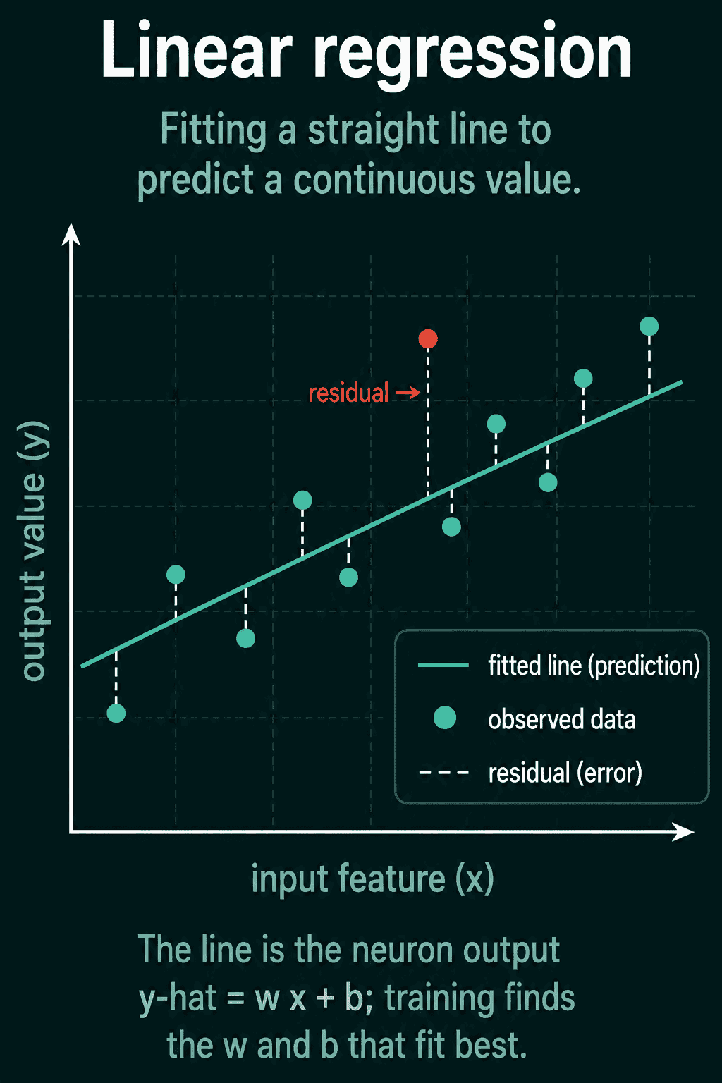
With one input, plotted as $x$ on the horizontal axis and the true output $y$ on the vertical axis, the model is a straight line through the data. The vertical gap between a data point and the line is that point's residual: how far the prediction is from the true value.

The model: $\hat{y} = wx + b$

For one input feature the model is

$$\hat{y} = wx + b$$

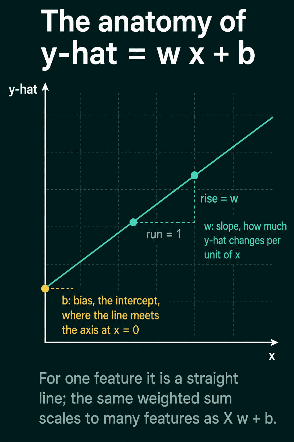
$\hat{y}$ (read "y hat") is the prediction, $x$ is the input, $w$ is the weight, and $b$ is the bias. The weight is the slope, how much $\hat{y}$ changes when $x$ goes up by 1. The bias is the intercept, the value of $\hat{y}$ when $x$ is 0, which shifts the whole line up or down. The same calculation, a weighted sum plus a bias, is what a single artificial neuron computes, so a linear regression model is one neuron with no threshold on its output.

Data points scattered around a fitted straight line, with a dashed vertical residual from each point to the line, and the caption noting that training finds the w and b that fit best.

A feature is one measurable property of a data point. A house might have its size, its age, and its distance from the city center as three features. With $d$ features, each one gets its own weight, and the prediction is the weighted sum plus the bias. For a whole dataset at once this is written with matrices:

$$\hat{\mathbf{y}} = \mathbf{X}\mathbf{w} + b$$

$\mathbf{X}$ is the input matrix with one row per example and one column per feature, so its shape is $(n, d)$ for $n$ examples. $\mathbf{w}$ is the weight vector of shape $(d, 1)$, and the matrix product $\mathbf{X}\mathbf{w}$ computes the weighted sum for every row in one step, giving predictions of shape $(n, 1)$.

The line y-hat equals w x plus b, with the slope w shown as the rise over a run of 1 and the bias b as the point where the line meets the vertical axis at x equals 0.

Scoring a line with mean squared error

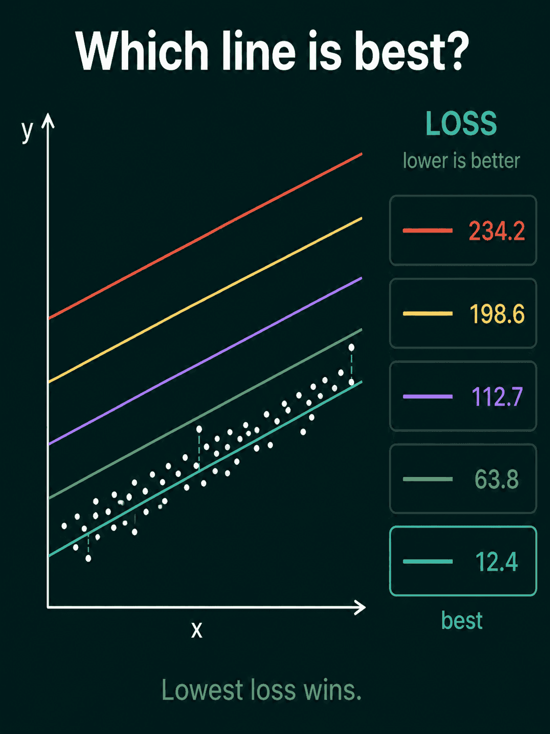
Every choice of $w$ and $b$ gives a different line, so training needs a single number that says how wrong a given line is. That number is the loss, and the formula that computes it is the loss function. The usual choice for linear regression is mean squared error (MSE): square each residual and average them.

$$\text{MSE} = \frac{1}{n} \sum_{i=1}^{n} (\hat{y}_i - y_i)^2$$

Squaring makes every residual positive, so errors above and below the line do not cancel, and it punishes a residual of 2 four times as much as a residual of 1. A lower MSE means a line closer to the data. Other regression losses score the same residuals differently: mean absolute error (MAE) averages their absolute values, root mean squared error (RMSE) takes the square root of MSE, and Huber loss is squared for small residuals and absolute for large ones. What is a loss function compares them and says when to pick each.

Five candidate lines over the same data, each with its loss: 234.2, 198.6, 112.7, 63.8, and 12.4 for the line running through the points, which is the best fit.

Training with gradients computed by hand

Gradient descent finds the best line by starting from any $w$ and $b$ and repeatedly moving them a small step in the direction that lowers the loss. That direction comes from the gradient, the derivative of the loss with respect to each parameter. For MSE, working through the derivative gives

$$\frac{\partial \text{MSE}}{\partial \mathbf{w}} = \frac{2}{n} \mathbf{X}^\top (\hat{\mathbf{y}} - \mathbf{y})$$

$$\frac{\partial \text{MSE}}{\partial b} = \frac{2}{n} \sum_{i=1}^{n} (\hat{y}_i - y_i)$$

$\mathbf{X}^\top$ is the transpose of $\mathbf{X}$, its rows turned into columns, so that multiplying it by the residuals sums each feature's contribution over all examples. Each step subtracts the gradient times a learning rate $\eta$, a small number that sets the step size: $\mathbf{w} \leftarrow \mathbf{w} - \eta , \partial \text{MSE}/\partial \mathbf{w}$, and the same for $b$.

The code below makes 200 fake houses with two features, size in hundreds of square meters and age in decades, and prices (in hundreds of thousands) that follow $3 \cdot \text{size} - 0.4 \cdot \text{age} + 1$ plus a little noise. Training should recover weights close to 3 and -0.4 and a bias close to 1.

1import torch
2 
3torch.manual_seed(0)
4n = 200
5X = torch.rand(n, 2) * torch.tensor([2.0, 5.0])    # size in 100 m², age in decades
6true_w = torch.tensor([[3.0], [-0.4]])
7y = X @ true_w + 1.0 + 0.1 * torch.randn(n, 1)     # price in 100k, plus noise
8 
9w = torch.zeros(2, 1)
10b = torch.zeros(1)
11lr = 0.05
12 
13for step in range(2000):
14    y_hat = X @ w + b                  # (200, 2) @ (2, 1) + (1,) -> (200, 1)
15    err = y_hat - y
16    loss = (err ** 2).mean()           # mean squared error
17    grad_w = 2 * X.T @ err / n         # dLoss/dw, shape (2, 1)
18    grad_b = 2 * err.mean()            # dLoss/db
19    w -= lr * grad_w
20    b -= lr * grad_b
21 
22print(w.squeeze().tolist(), b.item(), loss.item())
23# roughly [3.0153, -0.4011] 0.9954 0.0116

The learned weights are 3.015 and -0.401 and the bias is 0.995. The final loss of about 0.0116 is close to 0.01, the variance of the noise added to the prices, which is about as low as any line can go on this data.

The same model with nn.Linear

In practice PyTorch computes the gradients for you. nn.Linear(2, 1) holds a weight of shape (1, 2) and a bias, loss.backward() computes the gradient of the loss with respect to both, and the optimizer applies the update:

1model = torch.nn.Linear(2, 1)
2optimizer = torch.optim.SGD(model.parameters(), lr=0.05)
3loss_fn = torch.nn.MSELoss()
4 
5for step in range(2000):
6    loss = loss_fn(model(X), y)
7    optimizer.zero_grad()      # clear gradients from the previous step
8    loss.backward()            # compute d(loss)/d(weight) and d(loss)/d(bias)
9    optimizer.step()           # weight -= lr * grad, bias -= lr * grad
10 
11print(model.weight.squeeze().tolist(), model.bias.item())
12# roughly [3.0153, -0.4011] 0.9954

It lands on the same weights as the hand-written version, because it minimizes the same loss with the same update rule, even though nn.Linear starts from small random weights instead of zeros. This loop is the one used to train much larger networks, with a different model and loss inside it.

When to use it, and common mistakes

Linear regression is a reasonable first model whenever the target is a number: on small datasets it can train in seconds, and each weight says how much the prediction moves per unit of its feature. It fits poorly when the real relationship curves, for example when price rises faster than size, and a curved relationship needs extra features like $x^2$ or a nonlinear model.

Shape mismatch between predictions and targets. If y has shape (200,) while the model outputs (200, 1), then y_hat - y broadcasts to a (200, 200) matrix and the loss is silently wrong. nn.MSELoss prints a warning in this case, and y.unsqueeze(1) fixes it.
Features on very different scales. If one feature is in square meters (up to about 200) and another is a count of rooms (up to about 5), a learning rate small enough for the first is far too small for the second, and training either crawls or blows up to nan. Standardizing each feature to mean 0 and standard deviation 1 fixes this, and it is the first thing to try when the loss explodes.
Forgetting optimizer.zero_grad(). PyTorch adds new gradients to the old ones, so skipping it makes each step use the sum of every gradient so far.

Logistic regression uses the same weighted sum $\mathbf{X}\mathbf{w} + b$, passes it through a sigmoid to get a probability between 0 and 1, and is used for classification instead of predicting a number. The perceptron also computes a weighted sum plus a bias but outputs a hard 0 or 1, and is covered in what is a perceptron. The update rule used here is explained step by step in what is gradient descent.

QuiddityML teaches linear regression in Unit 1 of the ML Foundation track, with exercises that include ordering the lines of a LinearRegression class, spotting the bug in its forward pass, and tracing tensor shapes from an input of shape (16, 3) to the predictions (quiddityml.com).