23 September 2026 · 13 min read · fundamentalsloss functionspytorch
What is a loss function? MSE, cross-entropy, and when to use which
A loss function turns a model's predictions into one number that says how wrong they are, and training is the process of pushing that number down. This post explains why models need one, which loss to use for regression, binary, multi-class, and multi-label problems (and for a few other tasks), and how to use the loss on a proper validation split to evaluate a model.
A loss function takes a model's predictions and the correct answers and returns one number that says how wrong the predictions are. A loss of 0 means every prediction was exactly right, and a higher loss means worse predictions. Training a model means changing its weights until this number is as small as possible, so the loss is how you tell the model what "good" means. With the wrong loss, a model can train smoothly and still get good at the wrong thing.
What a loss function does
Say a model predicts house prices in hundreds of thousands of dollars. For four houses it predicts 3.1, 7.4, 1.9, and 5.2, and the real prices are 3.0, 8.0, 2.0, and 5.0. A loss function compares each prediction with its true value and combines all four differences into a single number.
The usual notation: $\hat y$ (read "y-hat") is a prediction, $y$ is the true value, and $\mathcal{L}(\hat y, y)$ is the loss computed from them. When the loss is averaged over a dataset of $n$ examples, $\hat y_i$ and $y_i$ are the prediction and true value for example $i$.
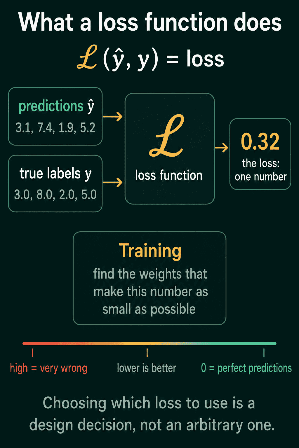
The picture shows the loss as 0.32 for these four houses. Which loss produced that number is covered in the regression section below, because different losses give different numbers for the same predictions.
Why a model needs a loss function
A model's weights are the numbers inside it that training adjusts. To improve, the model needs to know, for each weight, whether nudging it up or down makes the predictions better. The loss answers that. For every weight, training computes how much the loss changes when that weight changes slightly. That collection of rates is the gradient, and computing it for every weight at once is what backpropagation does. Then every weight takes a small step in the direction that lowers the loss, which is gradient descent. Repeat that over many batches of data and the loss goes down.
This puts two requirements on a loss:
- It is one number. Gradient descent lowers one quantity at a time. If you care about two things, such as getting the class right and getting the box position right in object detection, you add the two losses into one, usually with a weight on each.
- It changes smoothly with the weights. A tiny change to one weight has to produce a tiny, measurable change in the loss, or the gradient is zero and training has nothing to follow. Accuracy fails this test. Nudge one weight slightly and almost every prediction stays on the same side of the decision, so accuracy usually stays the same. That is why classifiers train on cross-entropy and report accuracy.
Losses for regression: predicting a number
Regression means predicting a continuous number: a price, a temperature, a delivery time. The four common losses all start from the error, $\hat y_i - y_i$, and differ in how they charge for it.
Mean squared error (MSE)
MSE squares each error and averages the squares:
$$\text{MSE} = \frac{1}{n}\sum_{i=1}^{n}(\hat y_i - y_i)^2$$
For the four houses, the errors are 0.1, −0.6, −0.1, and 0.2. The squares are 0.01, 0.36, 0.01, and 0.04, which sum to 0.42, so the MSE is 0.105.
Squaring makes large errors cost far more than small ones. An error of 1 costs 1, and an error of 3 costs 9. MSE is the loss you get if you assume the errors follow a bell-shaped normal distribution around the true value, and it is the usual default for regression. It is a poor choice when the data has outliers, because a single bad example can outweigh everything else. In PyTorch it is nn.MSELoss().
Root mean squared error (RMSE)
RMSE is the square root of MSE:
$$\text{RMSE} = \sqrt{\text{MSE}}$$
For the four houses that is $\sqrt{0.105} \approx 0.32$, the number in the picture above. RMSE is in the same units as the target (hundreds of thousands of dollars here), so it is easier to read than MSE. Minimizing RMSE and minimizing MSE lead to the same weights, so people usually train on MSE and report RMSE. PyTorch has no separate RMSE loss, so compute it as torch.sqrt(nn.functional.mse_loss(pred, y)).
Mean absolute error (MAE)
MAE averages the absolute errors instead of squaring them:
$$\text{MAE} = \frac{1}{n}\sum_{i=1}^{n}\lvert \hat y_i - y_i \rvert$$
For the four houses, that is (0.1 + 0.6 + 0.1 + 0.2) / 4 = 0.25. An error three times larger costs three times more, not nine times more, so outliers pull on the model much less.
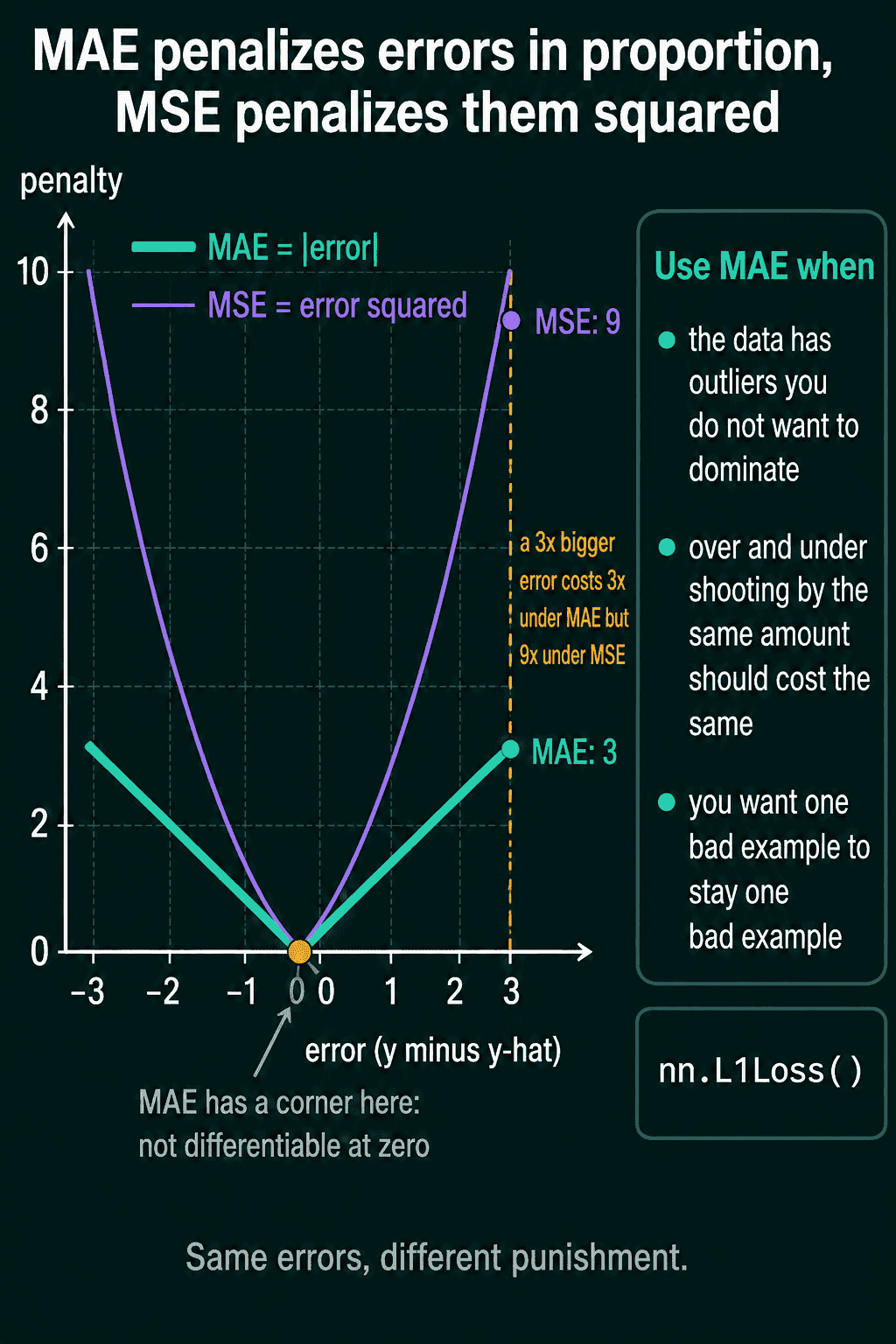
The difference shows up fast with one outlier. Add a fifth house predicted at 4.0 that actually sold for 14.0, an error of 10. MSE jumps from 0.105 to (0.42 + 100) / 5 ≈ 20.1, almost all of it from that one house. MAE goes from 0.25 to (1.0 + 10) / 5 = 2.2.
MAE has a corner at an error of 0, where it is not differentiable. PyTorch handles that point fine in practice, but the gradient has the same size whether the error is 0.01 or 10, so updates don't shrink as predictions get close to right. There is also a statistical difference: a model trained with MSE is pulled toward predicting the mean of the possible values, and one trained with MAE toward the median. In PyTorch MAE is nn.L1Loss().
Huber loss
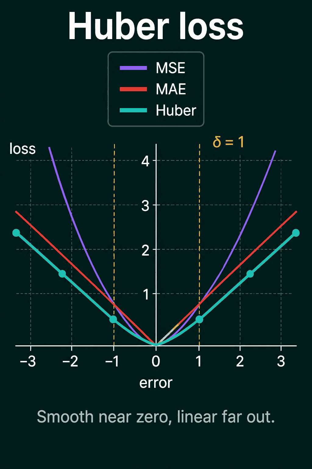
Huber loss is MSE for small errors and MAE for large ones. A setting $\delta$ (delta) marks where it switches. For an error $e = \hat y - y$:
$$L_\delta(e) = \tfrac{1}{2}e^2 \quad \text{if } |e| \le \delta$$
$$L_\delta(e) = \delta\left(|e| - \tfrac{1}{2}\delta\right) \quad \text{otherwise}$$
Near zero it behaves like MSE, so updates shrink as the prediction gets close, and far out it grows in a straight line like MAE, so outliers can't take over. It is a good choice for data that is mostly clean with some bad values. In PyTorch it is nn.HuberLoss(delta=1.0). nn.SmoothL1Loss(beta=1.0) is the same shape divided by beta, and is often used for bounding boxes in object detection.
1import torch
2import torch.nn as nn
3
4pred = torch.tensor([3.1, 7.4, 1.9, 5.2])
5target = torch.tensor([3.0, 8.0, 2.0, 5.0])
6
7print(nn.MSELoss()(pred, target))               # 0.105
8print(torch.sqrt(nn.MSELoss()(pred, target)))   # RMSE, 0.324
9print(nn.L1Loss()(pred, target))                # MAE, 0.25
10print(nn.HuberLoss(delta=1.0)(pred, target))    # 0.0525, all errors are under delta
Losses for binary classification: yes or no
Binary classification means choosing between two classes: spam or not spam, fraud or not fraud. The model outputs one number per example, called a logit, which can be any real number. The sigmoid function turns the logit $z$ into a probability $p$ between 0 and 1:
$$\sigma(z) = \frac{1}{1 + e^{-z}}$$
Here $p$ is the predicted probability that the example is in class 1, and the label $y$ is 1 or 0. Binary cross-entropy (BCE) is:
$$\text{BCE} = -\frac{1}{n}\sum_{i=1}^{n}\Big[y_i \log p_i + (1 - y_i)\log(1 - p_i)\Big]$$
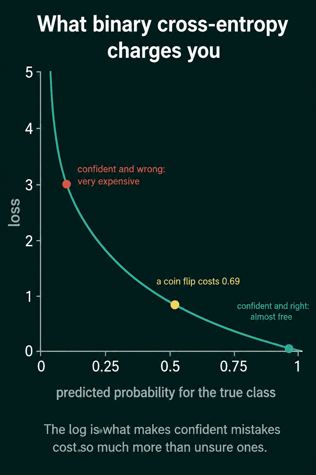
For each example only one of the two terms is active. If the label is 1, the loss is $-\log p$, and if the label is 0, it is $-\log(1-p)$. With a true label of 1, a prediction of $p = 0.9$ costs 0.105, a coin-flip $p = 0.5$ costs 0.693, $p = 0.1$ costs 2.303, and $p = 0.01$ costs 4.605.
The log is what makes a confident wrong answer expensive. Going from 0.1 to 0.01 on a true example doubles the loss, even though both predictions count as equally wrong on accuracy.
MSE on sigmoid outputs trains poorly. When the model is confidently wrong, the sigmoid is nearly flat, so MSE's gradient is tiny exactly when the model most needs to change. With BCE the gradient with respect to the logit works out to $p - y$, which stays large when the prediction is far off.
In PyTorch, use nn.BCEWithLogitsLoss() and pass it raw logits. It applies the sigmoid and the log together in a numerically stable way, which avoids the log(0) that nn.BCELoss on already-squashed probabilities can hit. For imbalanced data, pos_weight makes errors on the rare positive class cost more, and a common starting value is the number of negatives divided by the number of positives.
1logits = model(x).squeeze(-1)           # shape (batch,)
2y = y.float()                           # 0.0 or 1.0, same shape as logits
3loss_fn = nn.BCEWithLogitsLoss(pos_weight=torch.tensor(20.0))  # 1 positive per 20 negatives
4loss = loss_fn(logits, y)
Losses for multi-class classification: one of K
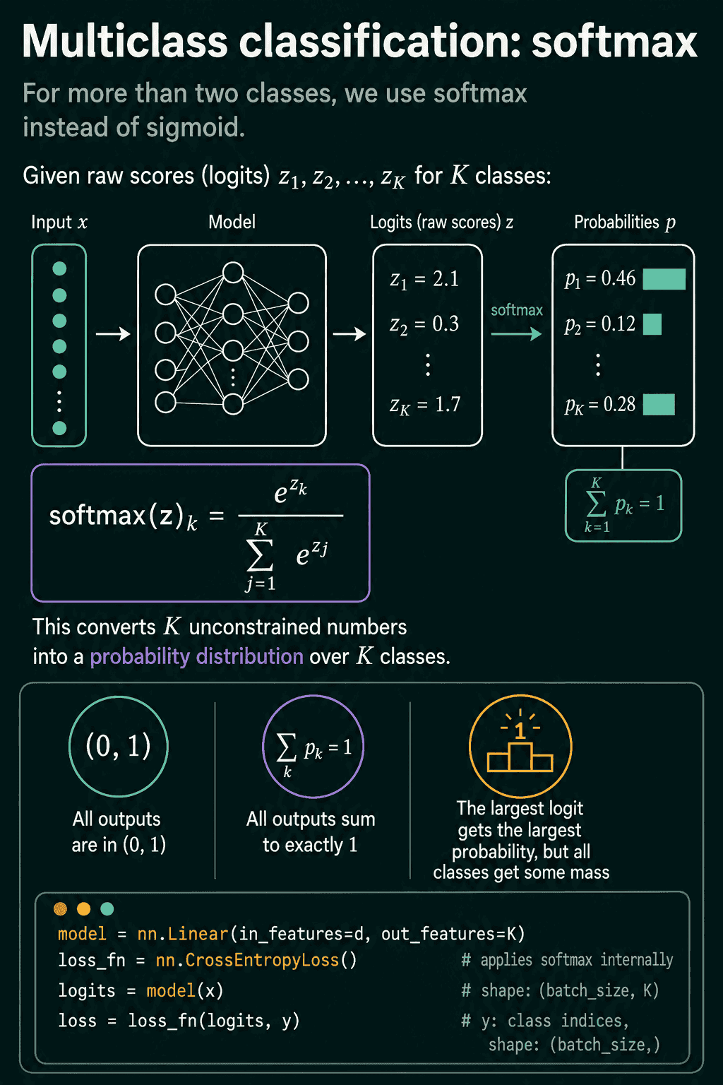
Multi-class classification means picking exactly one of $K$ classes: which digit, which species, which intent. The model outputs $K$ logits $z_1, \dots, z_K$, and softmax turns them into $K$ probabilities that are each between 0 and 1 and sum to 1:
$$\text{softmax}(z)k = \frac{e^{z_k}}{\sum{j=1}^{K} e^{z_j}}$$
Cross-entropy is the negative log of the probability the model gave to the correct class, averaged over examples. Writing $p_{i,y_i}$ for the probability that example $i$ got on its correct class $y_i$:
$$\text{CE} = -\frac{1}{n}\sum_{i=1}^{n}\log p_{i,y_i}$$
If the correct class got probability 0.46, the loss for that example is $-\log 0.46 \approx 0.78$. The probabilities on the wrong classes don't appear in the formula directly, but softmax ties them together, so raising the correct class's probability lowers the others.
The log has a reason beyond making confident mistakes expensive. The probability the model assigns to all the correct labels in a dataset is the product of the per-example probabilities, and the log turns that product into a sum. Minimizing cross-entropy is therefore the same as making the observed labels as probable as possible under the model, which is called maximum likelihood.
nn.CrossEntropyLoss() takes raw logits of shape (batch, K) and targets as class indices of dtype long with shape (batch,). It applies log-softmax internally, so the model's last layer should be a plain linear layer with no softmax. Two options are worth knowing:
label_smoothing=0.1moves a small share of the target away from the correct class and spreads it evenly over all classes. The model stops getting rewarded for pushing the correct probability all the way to 1, which often reduces overconfidence.weight=takes one weight per class and makes errors on rare classes cost more, the multi-class version ofpos_weight.
Losses for multi-label classification: several yes/no answers
In multi-label classification one example can have several labels at once, such as a photo that contains both a dog and a car. That is $K$ independent yes/no questions, so the model outputs $K$ logits and each one gets its own sigmoid and its own binary cross-entropy.
Softmax is the wrong choice here, because it forces the $K$ probabilities to sum to 1. A higher probability for "dog" would then push "car" down, even though both are in the photo. In PyTorch, use nn.BCEWithLogitsLoss() with a float target of 0s and 1s shaped (batch, K), the same shape as the logits.
Losses for other tasks
Most other losses are built from the ones above, applied to a different kind of output.
- Language models. Predicting the next token is multi-class classification over the vocabulary, done at every position in the text. The loss is cross-entropy averaged over all positions. Perplexity, a number often reported for language models, is $e$ raised to that average cross-entropy.
- Image segmentation. Labeling every pixel with a class is classification per pixel, so the base loss is cross-entropy averaged over pixels.
nn.CrossEntropyLossaccepts logits shaped(batch, K, H, W)and targets shaped(batch, H, W). When the object covers only a small share of the image, Dice loss is often added. It measures the overlap between the predicted mask and the true mask, 1 minus twice the overlap divided by the total size of both, so a small object isn't drowned out by the many background pixels around it. - Object detection. A detector predicts what each object is and where its box is. The loss is a sum: cross-entropy for the class, plus an L1, Huber, or box-overlap loss for the box coordinates.
- Embeddings and similarity search. These models are trained so that similar items end up close together. A triplet loss takes an anchor, a matching example, and a non-matching one, and charges the model unless the anchor is closer to the match than to the non-match by at least a margin: $\max(0,; d(a,p) - d(a,n) + \text{margin})$, where $d$ is the distance. Contrastive losses such as InfoNCE treat the matching item as the correct class among everything else in the batch and apply cross-entropy over similarity scores. PyTorch has
nn.TripletMarginLoss(). - Distillation. Training a small student model to copy a large teacher uses KL divergence, which measures how different the student's probability distribution is from the teacher's.
nn.KLDivLoss()expects the student's log-probabilities as input. - Heavy class imbalance. Focal loss multiplies cross-entropy by a factor that shrinks for examples the model already gets right with high confidence, so training focuses on the hard ones. It is common in object detection.
Which loss to use
| task | output layer | loss | PyTorch |
|---|---|---|---|
| regression | one linear output | MSE, MAE, or Huber | nn.MSELoss, nn.L1Loss, nn.HuberLoss |
| binary | one logit | binary cross-entropy | nn.BCEWithLogitsLoss |
| multi-class | K logits | cross-entropy | nn.CrossEntropyLoss |
| multi-label | K logits | binary cross-entropy per label | nn.BCEWithLogitsLoss |
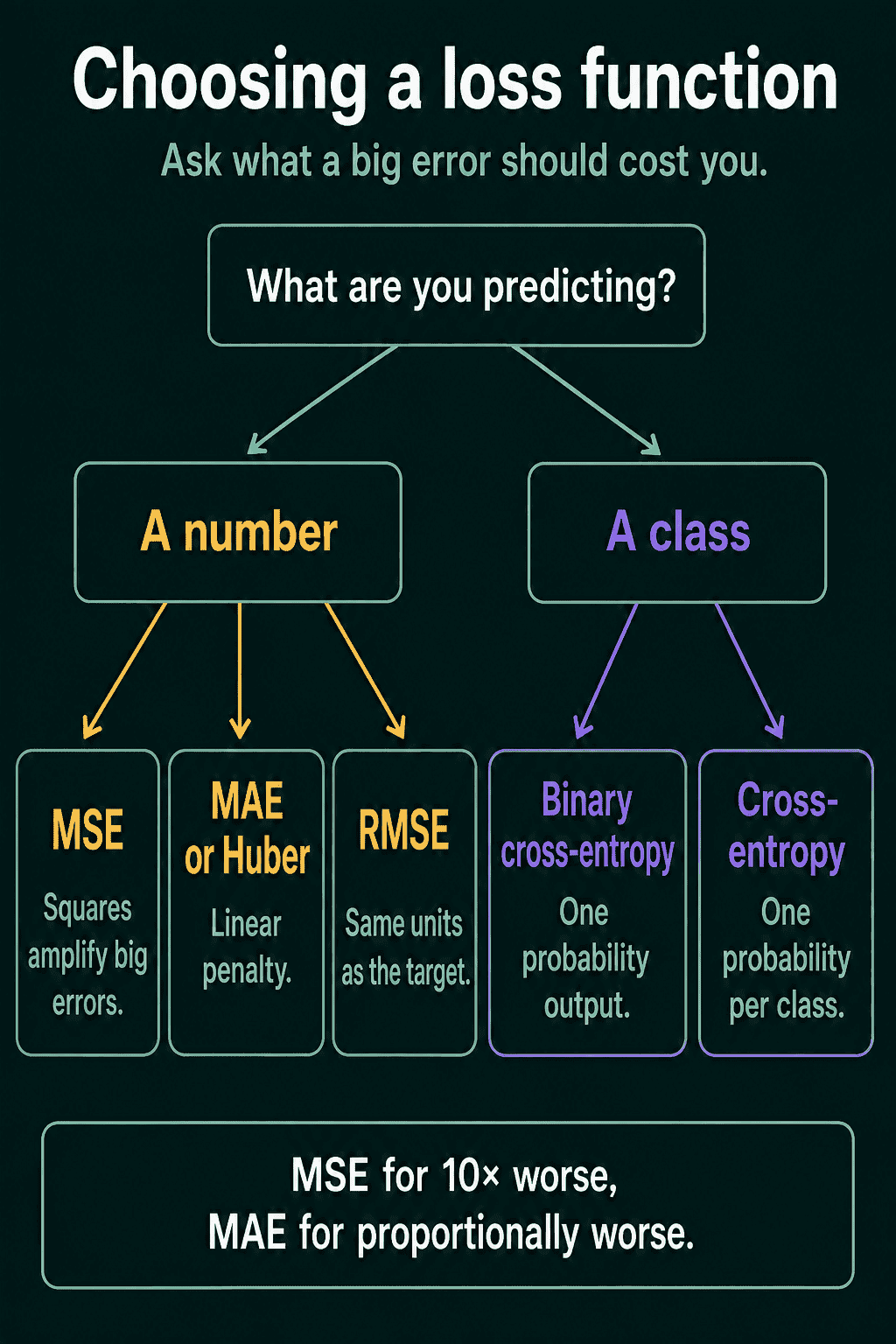
For regression, the choice comes down to what a big error should cost. Use MSE when a big miss really is much worse than a small one, MAE or Huber when big misses are mostly bad data, and report RMSE or MAE in the target's units either way.
Using the loss to evaluate a model
The loss on the training data only says how well the model fits examples it has already seen. A model can drive training loss close to 0 by memorizing, which is overfitting, and still do badly on new data. To see how it does on new data, you need a split.
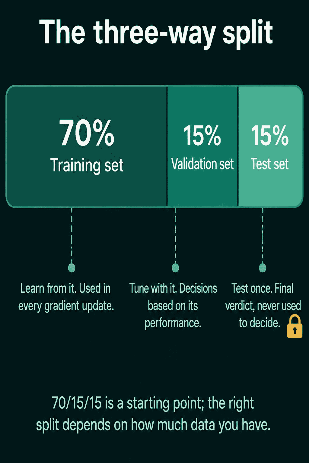
- The training set is what the weights learn from. Every gradient update uses it.
- The validation set is held out from training and used for decisions: which learning rate, which model size, when to stop.
- The test set is held out from everything and scored once, at the end, to report how the final model does.
After each epoch, compute the same loss on the validation set with the model in evaluation mode and gradients turned off:
1model.eval()
2total, count = 0.0, 0
3with torch.no_grad():
4    for x, y in val_loader:
5        logits = model(x)
6        total += loss_fn(logits, y).item() * len(y)
7        count += len(y)
8val_loss = total / count
9model.train()
Then compare the two curves. Both falling means the model is learning. Training loss still falling while validation loss rises means overfitting. Both staying high means underfitting, a model too simple or trained too little to fit even the training data. The overfitting vs underfitting post shows what each curve looks like, the bias-variance tradeoff post explains why they happen, and regularization covers the fixes for overfitting.
Validation loss and a metric like accuracy can disagree. Validation loss can rise while accuracy holds steady, because the model grows more confident on the examples it already gets wrong, and cross-entropy charges heavily for confident mistakes while accuracy only counts right and wrong. Track both: the loss tells you how training is going, and the task metric (accuracy, F1, RMSE in real units) tells you what people using the model will see.
A validation score is only as good as the split behind it:
- Split before fitting anything on the data. Normalization statistics, vocabularies, and imputation values come from the training set only. Computing them on all the data leaks information from the validation and test sets into training.
- Split by group when examples are related. All photos of one patient, all messages from one user, or all frames from one video go into the same split. Otherwise the model can score well by recognizing the person instead of learning the task.
- Split by time when you will predict the future. Train on earlier data and validate on later data, the same direction the model will be used in.
- Remove duplicates across splits. A near-copy of a training example in the test set inflates the score.
- Keep class proportions similar in each split when a class is rare, so the validation set has enough of it to measure.
- Use the test set once. Every decision made by looking at the test score makes it a little more optimistic.
Losses are only comparable on the same data, with the same loss function and the same reduction. A validation loss of 0.4 on one split says nothing about a 0.5 on a different split.
Common mistakes
- Softmax before
nn.CrossEntropyLoss. The loss applies log-softmax itself, so softmax gets applied twice and training slows down or stalls. Feed it raw logits. - Sigmoid before
nn.BCEWithLogitsLoss. Same problem with the binary version. - Wrong target dtype or shape.
nn.CrossEntropyLosswantslongclass indices shaped(batch,).nn.BCEWithLogitsLosswants floats with the same shape as the logits. For MSE, predictions shaped(batch, 1)against targets shaped(batch,)broadcast into a(batch, batch)grid and give a wrong loss with only a warning. - MSE for classification. It trains slowly on sigmoid or softmax outputs for the reason covered in the binary section.
reduction="sum"without adjusting the learning rate. A summed loss grows with batch size, so changing the batch size changes the step size.- Reading training loss below validation loss as a bug. Dropout is active when the training loss is computed and off during validation, so validation loss can legitimately come out lower.
- Tuning on the test set. Pick settings on validation and score the test set once.
If the loss isn't going down at all, the loss not decreasing checklist walks through the usual causes.
QuiddityML teaches loss functions in the first unit of its ML Foundation track, and the exercises include picking a loss for house prices with a few extreme mansions, writing Huber loss and binary cross-entropy from scratch with tensor operations, and spotting what goes wrong when sigmoid outputs are passed to BCEWithLogitsLoss.