25 September 2026 · 7 min read

What is a perceptron? From the original perceptron to the modern neuron

A perceptron is the simplest artificial neuron: it weighs its inputs, adds them up, and outputs 0 or 1. This post explains how it works, how it learns, why modern neurons output a real number instead, and why one neuron can never solve XOR.

A perceptron is the simplest artificial neuron: it multiplies each input by a weight, adds the results together with one extra number, and outputs 1 if the total is above zero and 0 otherwise. Most neural networks are built from units that do almost the same calculation, so the perceptron's strengths and its one big limit carry into the networks built from it.

Where the idea came from

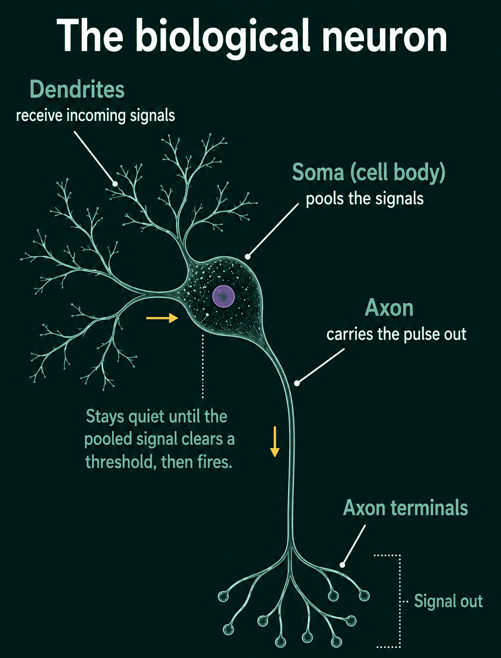
A biological neuron receives signals from other neurons through its dendrites, pools them in the cell body, and stays quiet until the pooled signal clears a threshold. When it does, the neuron fires a pulse down its axon to the neurons it connects to.

A biological neuron with dendrites receiving signals, the cell body pooling them, and the axon carrying a pulse out once the pooled signal clears a threshold.

In 1943, Warren McCulloch and Walter Pitts turned that idea into a very small piece of math: a few inputs that are each on or off, and one output that turns on when enough inputs are on. A handful of these units can compute logic gates like AND, OR, and NOT, but a person has to choose the settings by hand.

In 1957, Frank Rosenblatt made the idea learnable. His perceptron gives each input its own weight and adjusts those weights from examples, so the same unit can learn different rules from different data.

How a perceptron makes a decision

A perceptron takes a list of numbers as input. Call them $x_1, x_2, \ldots, x_n$. For a spam filter, $x_1$ could be the number of links in an email and $x_2$ the number of words in capital letters.

Each input $x_i$ has a weight $w_i$, a number that says how much that input pushes the decision. A large positive weight means more of that input makes a 1 more likely, and a negative weight means it makes a 1 less likely. There is also one bias $b$, a number added to the total that shifts where the cutoff sits, independent of the inputs.

The perceptron multiplies each input by its weight, adds them up, adds the bias, and applies a hard threshold: output 1 if the total is above zero, and 0 otherwise. Written out, with $\hat{y}$ (read "y hat") as the prediction:

$$\hat{y} = \begin{cases} 1 & \text{if } \sum_i w_i x_i + b > 0 \ 0 & \text{otherwise} \end{cases}$$

The sum $\sum_i w_i x_i$ means "multiply each input by its weight and add the products". The weights and the bias are the perceptron's parameters, the numbers it learns from data.

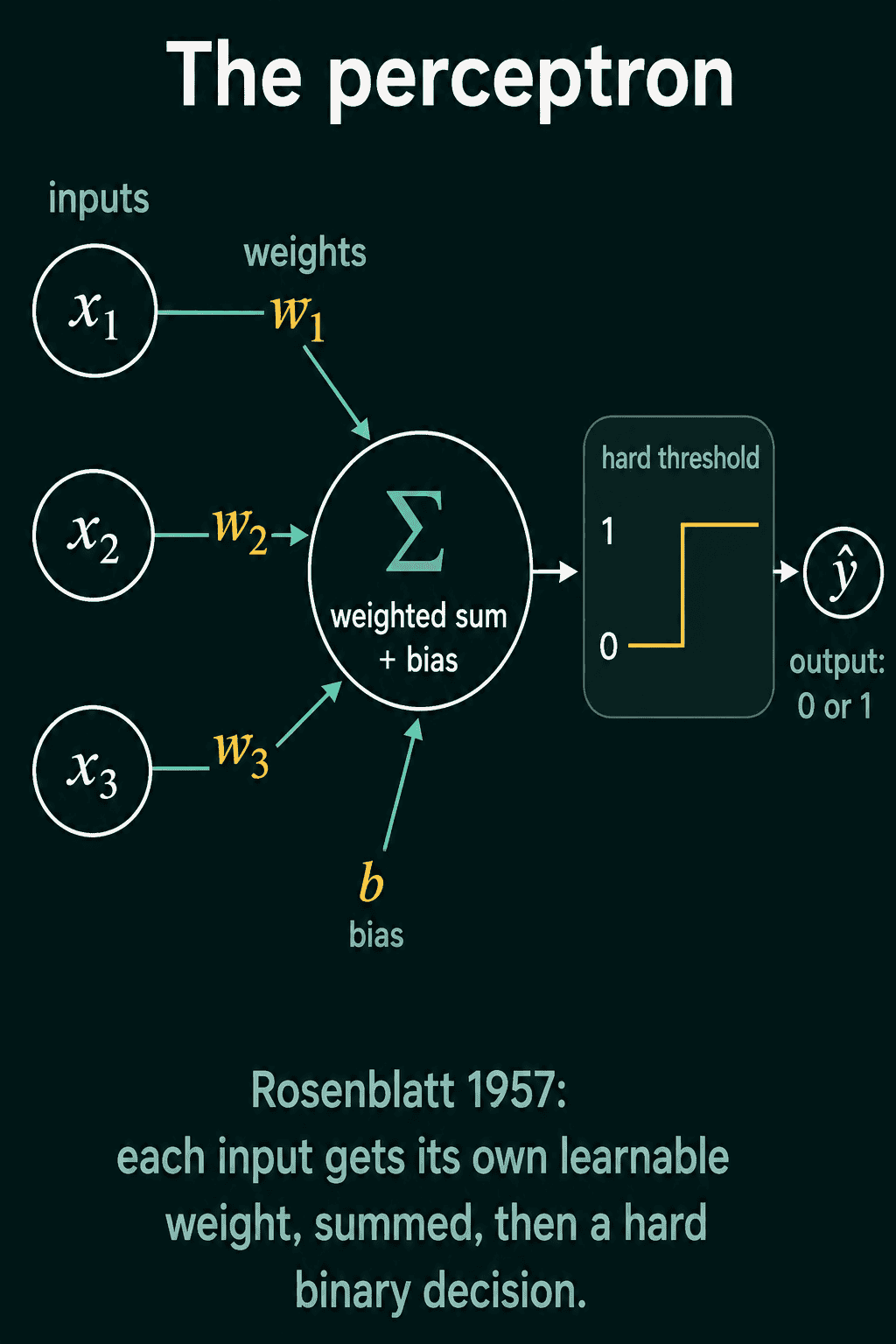
A perceptron with three inputs, each multiplied by its own weight, summed with a bias, then passed through a hard threshold that outputs 0 or 1.

Because the output is one of two labels, the perceptron is a classifier: it sorts each input into one of two classes, like spam or not spam.

How a perceptron learns

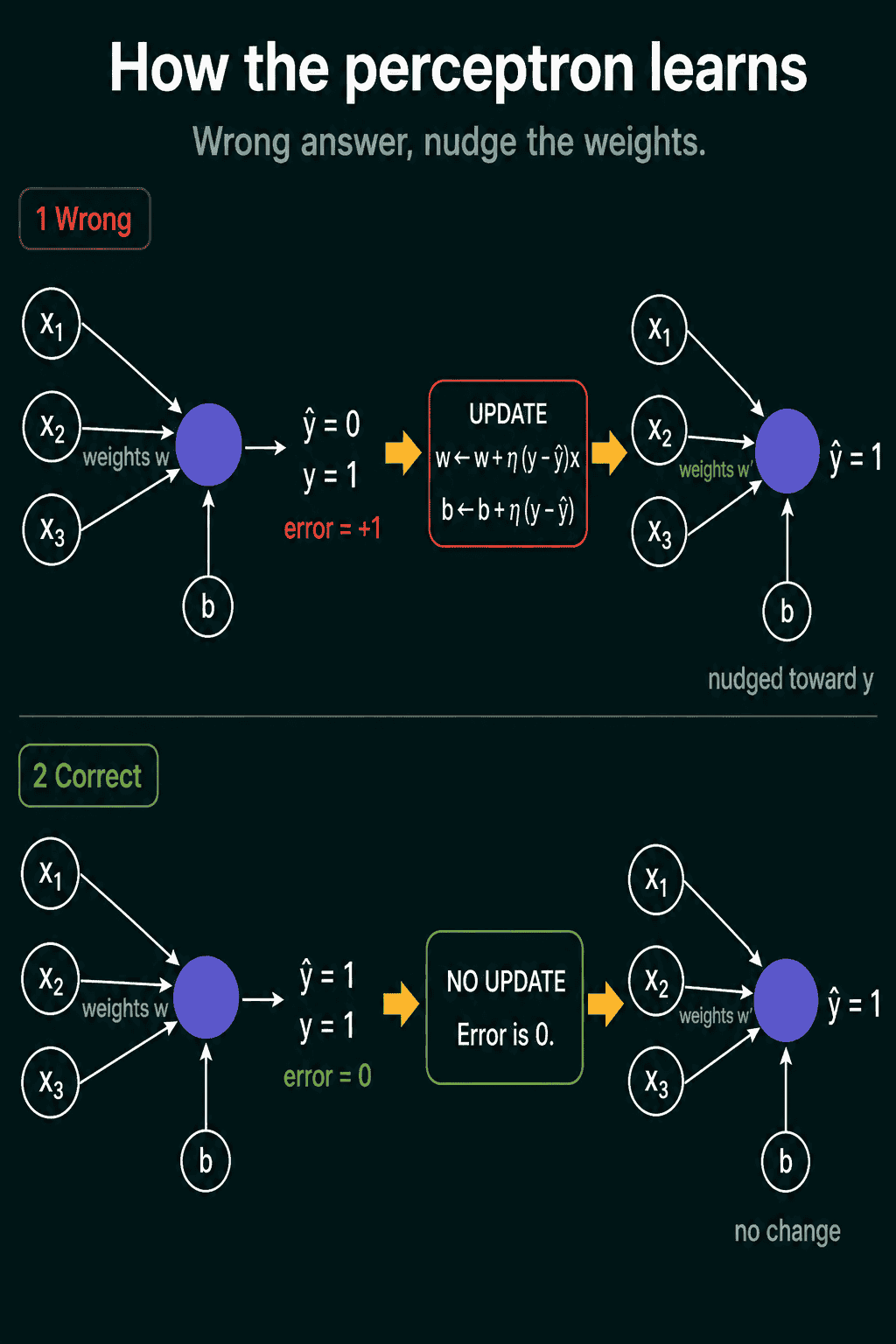
Training starts with the weights and bias at zero (or small random values) and goes through the labeled examples one at a time. For each example, the perceptron makes a prediction $\hat{y}$ and compares it with the true label $y$. If they match, nothing changes. If they differ, it nudges each weight and the bias:

$$w_i \leftarrow w_i + \eta , (y - \hat{y}) , x_i$$

$$b \leftarrow b + \eta , (y - \hat{y})$$

The arrow $\leftarrow$ means "becomes": take the current value, add the adjustment, and store the result. $\eta$ (the Greek letter eta) is the learning rate, a small number like 0.1 that sets the size of each nudge. Since $y$ and $\hat{y}$ are both 0 or 1, the error $y - \hat{y}$ is 0 when the prediction is right, +1 when the perceptron said 0 but should have said 1, and -1 in the opposite case. Multiplying by $x_i$ means an input that was 0 on this example leaves its weight alone, because it did not contribute to the mistake.

Two cases of the perceptron learning rule: a wrong prediction produces an error of +1 and the weights are nudged toward the true label, and a correct prediction produces an error of 0 and nothing changes.

If some straight line (or flat plane, with more inputs) can separate the two classes, this rule is guaranteed to find one after a finite number of mistakes. That result is the perceptron convergence theorem.

A perceptron in PyTorch

This code trains a perceptron with the rule above on two logic gates. AND outputs 1 only when both inputs are 1. XOR (exclusive or) outputs 1 when exactly one input is 1.

1import torch
2 
3X = torch.tensor([[0., 0.], [0., 1.], [1., 0.], [1., 1.]])
4y_and = torch.tensor([0., 0., 0., 1.])
5y_xor = torch.tensor([0., 1., 1., 0.])
6 
7def train_perceptron(X, y, lr=0.1, epochs=20):
8    w = torch.zeros(X.shape[1])
9    b = torch.tensor(0.0)
10    for _ in range(epochs):
11        for x_i, y_i in zip(X, y):
12            y_hat = (x_i @ w + b > 0).float()     # hard 0-or-1 decision
13            w += lr * (y_i - y_hat) * x_i          # no change when y_hat == y_i
14            b += lr * (y_i - y_hat)
15    return w, b
16 
17for name, y in [("AND", y_and), ("XOR", y_xor)]:
18    w, b = train_perceptron(X, y)
19    preds = (X @ w + b > 0).float()
20    print(name, "predicted", preds.tolist(), "target", y.tolist())
21 
22# AND predicted [0.0, 0.0, 0.0, 1.0] target [0.0, 0.0, 0.0, 1.0]
23# XOR predicted [1.0, 1.0, 0.0, 0.0] target [0.0, 1.0, 1.0, 0.0]

x_i @ w is the dot product, the same multiply-and-add as $\sum_i w_i x_i$. The perceptron learns AND perfectly and gets two of the four XOR cases wrong, and raising epochs does not fix XOR.

Why a perceptron cannot learn XOR

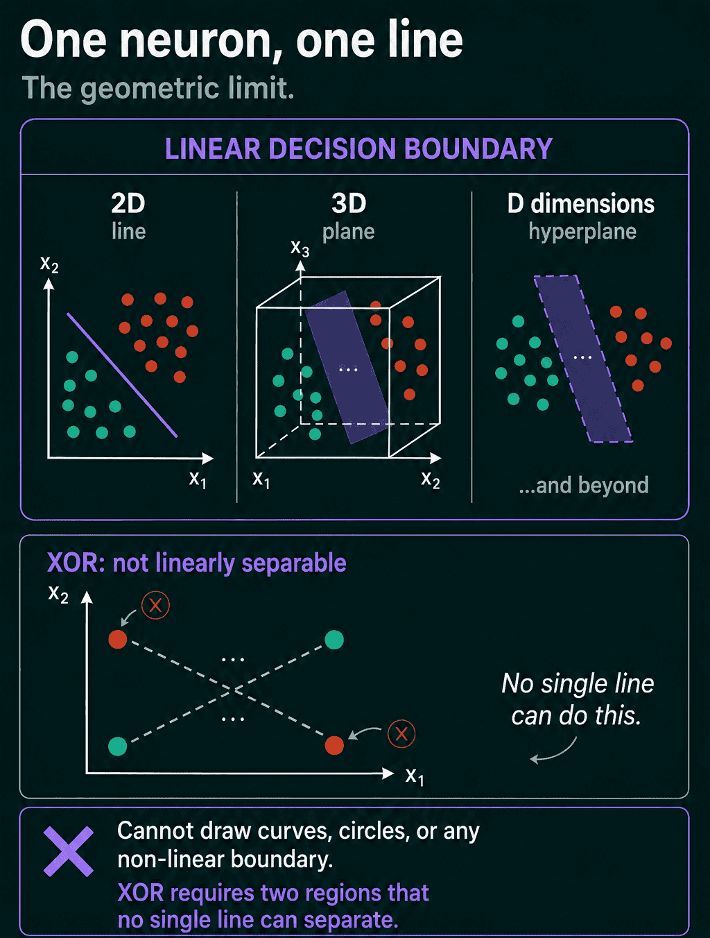
The perceptron outputs 1 exactly where $\sum_i w_i x_i + b > 0$. With two inputs, the points where that total is exactly zero form a straight line, so the perceptron splits the input plane into two halves: 1 on one side, 0 on the other. That line is its decision boundary.

For AND, one line works: put it so the corner $(1, 1)$ is on one side and the other three corners are on the other. For XOR, the 1s sit at $(0, 1)$ and $(1, 0)$, on one diagonal, and the 0s at $(0, 0)$ and $(1, 1)$, on the other. Any straight line that puts both 1s on one side also puts at least one 0 there. Classes that one straight line can separate are called linearly separable, and XOR is not.

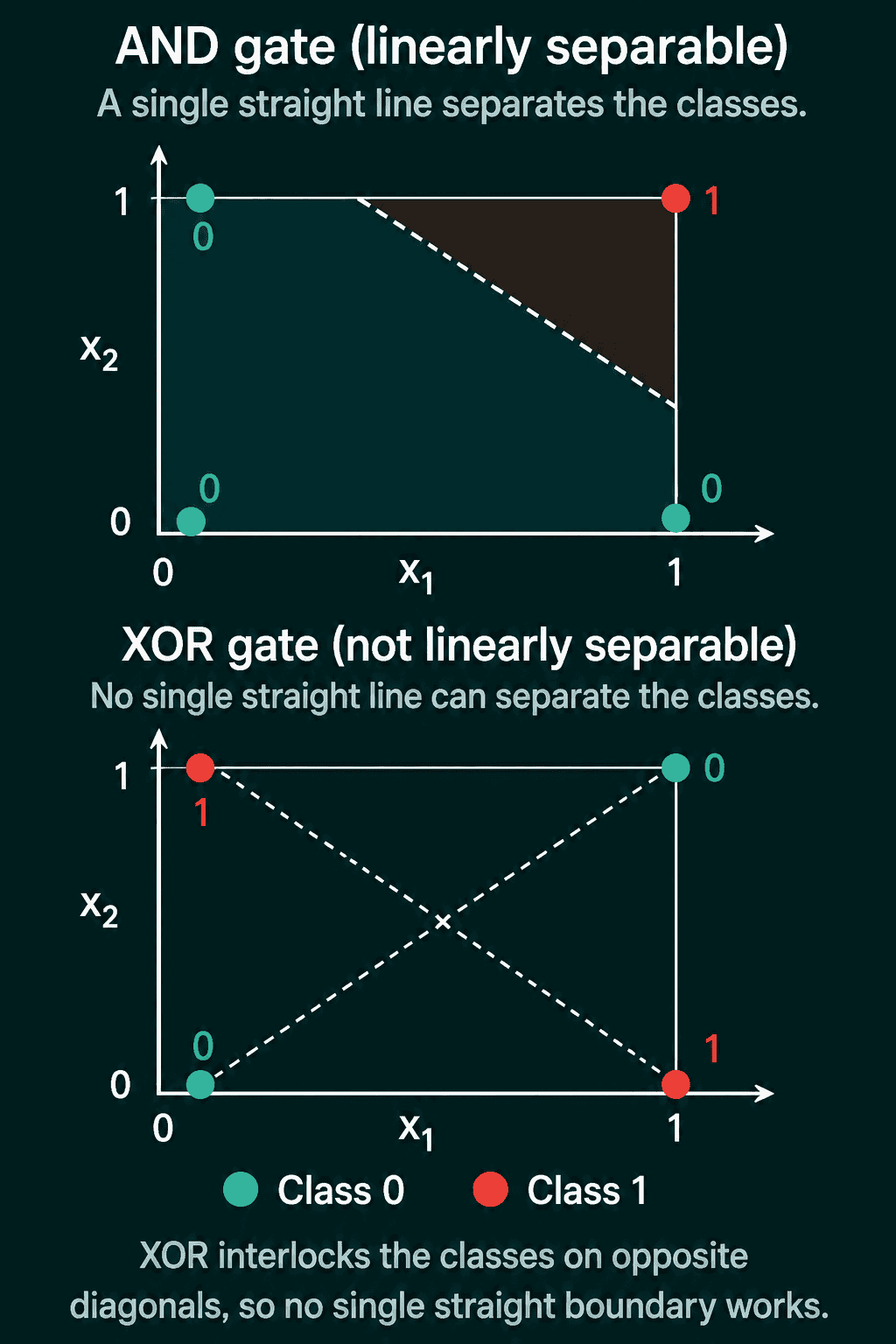
The AND gate, where one straight dashed line separates the single class-1 corner from the three class-0 corners, and the XOR gate, where the classes sit on opposite diagonals and no single straight line separates them.

This is a limit of the shape of the boundary, so more data or more training cannot fix it. In 1969, Marvin Minsky and Seymour Papert's book Perceptrons worked out this limit in detail.

The modern artificial neuron

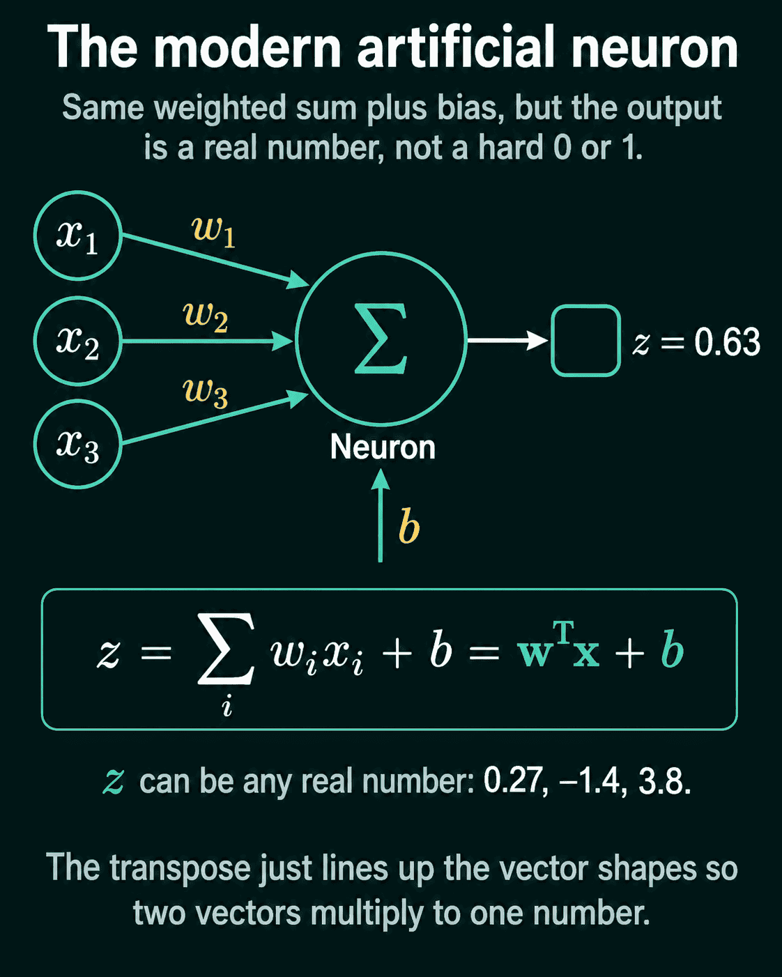
A modern neuron keeps the weighted sum and bias and drops the hard threshold, so its output is a real number:

$$z = \sum_i w_i x_i + b = \mathbf{w}^\top \mathbf{x} + b$$

Here $\mathbf{w}$ and $\mathbf{x}$ are the weights and inputs written as vectors (lists of numbers), and $\mathbf{w}^\top \mathbf{x}$ is their dot product. The $\top$ stands for transpose, which turns $\mathbf{w}$ from a column into a row so that multiplying the two vectors gives a single number. The output $z$ can be any real number, such as 0.27, -1.4, or 3.8.

The modern artificial neuron: the same weighted sum plus bias, with a real-valued output z such as 0.63 instead of a hard 0 or 1.

In PyTorch, nn.Linear holds the weights and bias and computes $z$ for a whole batch at once:

1import torch.nn as nn
2 
3neuron = nn.Linear(2, 1)   # 2 inputs, 1 output
4z = neuron(X)              # X from above has shape (4, 2), so z has shape (4, 1)

What a real-valued output adds

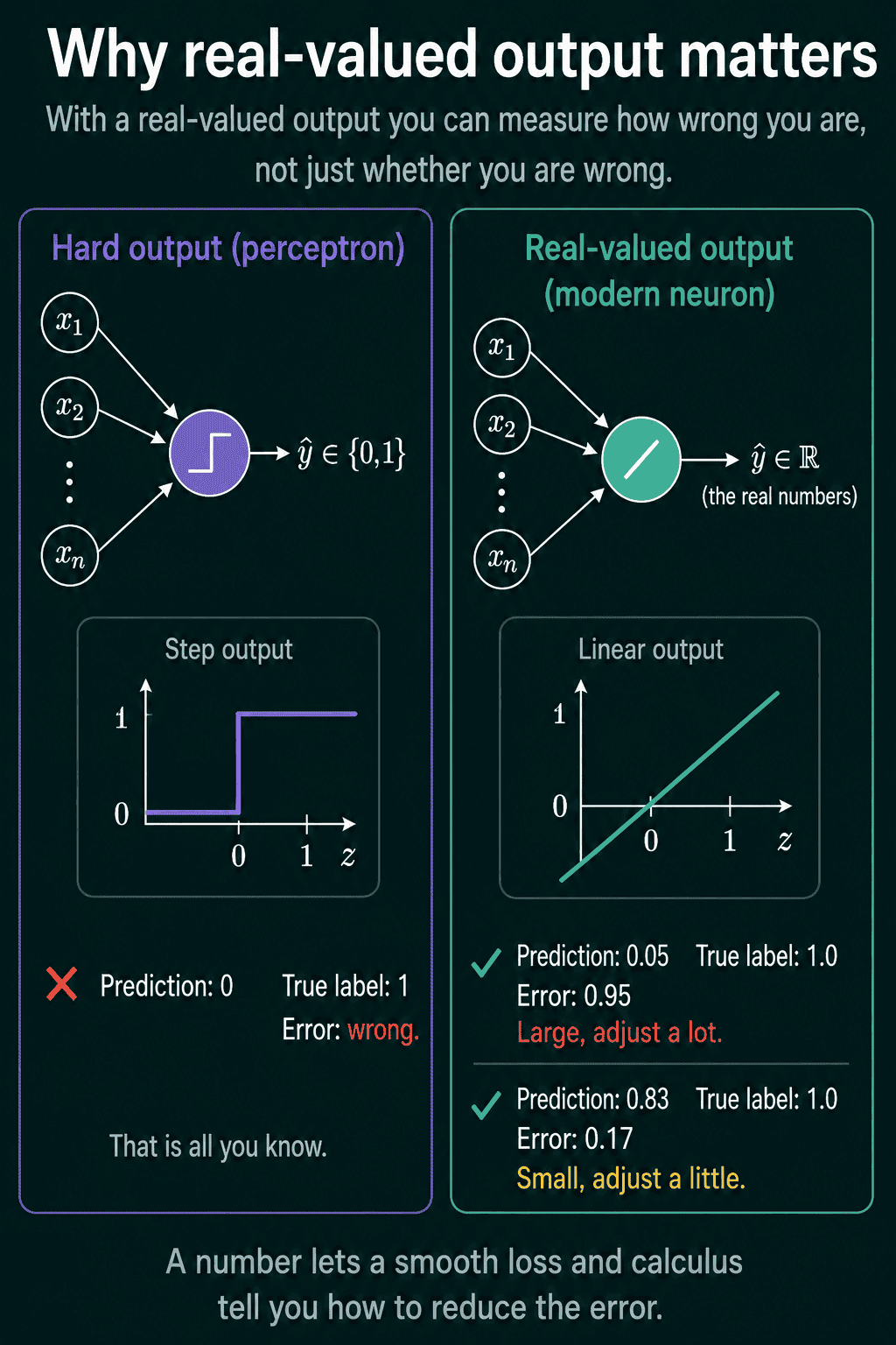
With a hard 0 or 1, the only thing a wrong prediction tells you is that it was wrong. With a real number you can measure how wrong: a prediction of 0.05 for a true label of 1.0 is off by 0.95, while 0.83 is off by only 0.17.

That measurement is what gradient-based training needs. A loss function turns the gap between predictions and labels into one number, and gradient descent adjusts every weight in the direction that makes that number smaller. The hard threshold blocks this, because its output does not change at all under a small change to a weight, so the gradient (the slope that says which way to move each weight) is zero almost everywhere.

A side-by-side of a hard step output, where a wrong prediction only says "wrong", and a linear output, where an error of 0.95 means adjust a lot and an error of 0.17 means adjust a little.

One neuron, one line

Dropping the threshold does not remove the geometric limit. A single neuron, whether it is the original perceptron, a modern linear neuron, or a neuron followed by a sigmoid (which is logistic regression), still separates classes with one linear boundary: a line with two inputs, a flat plane with three, and a hyperplane (the same flat cut in more dimensions) beyond that. It cannot draw a curve or a circle, so XOR stays out of reach.

A linear decision boundary as a line in 2D, a plane in 3D, and a hyperplane in higher dimensions, with XOR shown as not linearly separable.

The fix is to stack neurons into layers, with a nonlinear activation function between layers. A network with one hidden layer of two neurons can already solve XOR, because each hidden neuron draws its own line and the output neuron combines the two regions. That stacked design is the multilayer perceptron, and the choice of activation function is covered in the activation functions roadmap.

Common mistakes

Forgetting the bias. Without $b$, the decision boundary has to pass through the origin. For AND, that would need $w_1 \le 0$ and $w_2 \le 0$ (so $(0, 1)$ and $(1, 0)$ give 0) together with $w_1 + w_2 > 0$ (so $(1, 1)$ gives 1), which no pair of weights can satisfy.
Training longer on data that is not linearly separable. If a perceptron keeps making mistakes after many passes, check whether any straight line could separate the classes before tuning the learning rate.
Treating the perceptron as a probability model. A 1 from a perceptron carries no confidence. For a probability between 0 and 1, put a sigmoid on $z$ and train with a loss, which is logistic regression.

Logistic regression is a modern neuron with a sigmoid on its output, trained with gradient descent instead of the perceptron rule. It still draws one straight boundary. The multilayer perceptron stacks layers of neurons with nonlinear activations, which is what lets it fit boundaries like XOR's. Linear regression uses the same $z = \mathbf{w}^\top \mathbf{x} + b$ to predict a number instead of a class.

QuiddityML teaches the perceptron and the modern neuron in Unit 1 of the ML Foundation track, with exercises that include ordering the lines of a Perceptron class, tracing tensor shapes through its forward pass, and predicting what happens when a perceptron is trained on XOR for 10,000 epochs (quiddityml.com).