By Sagi Shaier · 14 October 2026 · 7 min read
Local minima and saddle points in deep learning
How to find the points where a function's gradient is zero, tell a minimum from a maximum or a saddle with the second-derivative test, and see in PyTorch why gradient descent can stall at a saddle.
A critical point of a function is a point where its gradient is zero, so the surface is flat in every direction right there. Gradient descent stops moving when it lands on one, which makes critical points the places where training can come to rest. Only some of them are minima. Others are saddle points, where the loss goes up in some directions and down in others, and in losses with many parameters they can be a common obstacle.
What a critical point is
The gradient $\nabla f(x)$ is the vector of partial derivatives of $f$. Each partial derivative is the slope along one input while the other inputs stay fixed. The gradient points in the direction where $f$ increases fastest, and gradient descent steps the other way. Each step is the gradient times a small number, so a smaller gradient gives a smaller step. When every partial derivative is zero at once,
$$\nabla f(x) = 0$$
the step is zero and gradient descent stops moving. Such a point is a critical point.
Take $f(x, y) = x^3 - 3x - y^3 + 3y$. Its partial derivatives are
$$\frac{\partial f}{\partial x} = 3x^2 - 3$$
$$\frac{\partial f}{\partial y} = -3y^2 + 3$$
The first is zero when $x = 1$ or $x = -1$. The second is zero when $y = 1$ or $y = -1$. So the function has four critical points: $(1, 1)$, $(1, -1)$, $(-1, 1)$ and $(-1, -1)$. The surface is flat at all four, and they turn out to be three different kinds of point.
Three kinds of critical point
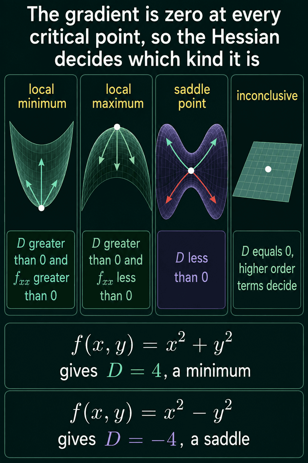
A flat point can be the bottom of a valley, the top of a hill, or neither:
- A local minimum is lower than every point close to it. The function curves upward in every direction around it.
- A local maximum is higher than every point close to it. The function curves downward in every direction around it.
- A saddle point is a critical point that is neither. Step off it in one direction and $f$ rises. Step off in another and $f$ falls.
The second-derivative test
The second derivatives say which way the function curves. Write $f_{xx}$ for the second derivative in $x$ and $f_{yy}$ for the second derivative in $y$. The mixed one $f_{xy}$ takes one derivative in $x$ and one in $y$. Together they form the Hessian matrix, and the discriminant combines them into one number:
$$D = f_{xx} f_{yy} - f_{xy}^2$$
At a critical point:
- $D > 0$ and $f_{xx} > 0$: local minimum.
- $D > 0$ and $f_{xx} < 0$: local maximum.
- $D < 0$: saddle point.
- $D = 0$: the test is inconclusive, and terms beyond the second derivatives decide.
For $f(x, y) = x^3 - 3x - y^3 + 3y$, the second derivatives are $f_{xx} = 6x$, $f_{yy} = -6y$ and $f_{xy} = 0$. Plugging in each critical point:
| Point | $f_{xx}$ and $f_{yy}$ | $D$ | Kind |
|---|---|---|---|
| $(1, -1)$ | $6$ and $6$ | $36$ | local minimum |
| $(-1, 1)$ | $-6$ and $-6$ | $36$ | local maximum |
| $(1, 1)$ | $6$ and $-6$ | $-36$ | saddle point |
| $(-1, -1)$ | $-6$ and $6$ | $-36$ | saddle point |
The function value is $-4$ at the minimum and $4$ at the maximum. At both saddles it is $0$. From $(1, 1)$, moving along $x$ raises $f$ because $f_{xx} = 6$ is positive, and moving along $y$ lowers it because $f_{yy} = -6$ is negative.
Why the mixed term counts
Upward curvature along both axes is not enough on its own. For $f(x, y) = x^2 + 3xy + y^2$, the gradient $(2x + 3y,\ 3x + 2y)$ is zero only at the origin. There $f_{xx} = 2$ and $f_{yy} = 2$ are both positive. The mixed term $f_{xy} = 3$ changes the answer:
$$D = 2 \cdot 2 - 3^2 = -5$$
so the origin is a saddle. Along the line $y = -x$ the function is $x^2 - 3x^2 + x^2 = -x^2$, which falls as you move away from the origin in either direction.
When the test says nothing
$D = 0$ happens when the second derivatives are too small to decide. The functions $x^4 + y^4$ and $x^4 - y^4$ both have a critical point at the origin. Every second derivative is zero there, so $D = 0$ for both. The first is a minimum, since it is never negative. The second is a saddle, since it rises along $x$ and falls along $y$. A $D = 0$ result means look further. It does not mean the point is a saddle.
Classifying critical points in code
hessian builds the matrix of second derivatives at a point, and classify_critical_point reads three of its entries:
1import torch
2from torch.autograd.functional import hessian
3
4def f(p):
5    x, y = p
6    return x ** 3 - 3 * x - y ** 3 + 3 * y
7
8def classify_critical_point(f_xx, f_xy, f_yy):
9    D = f_xx * f_yy - f_xy ** 2
10    if D > 0 and f_xx > 0:
11        return "local minimum"
12    if D > 0 and f_xx < 0:
13        return "local maximum"
14    if D < 0:
15        return "saddle point"
16    return "inconclusive"
17
18for point in [(1.0, 1.0), (1.0, -1.0), (-1.0, 1.0), (-1.0, -1.0)]:
19    p = torch.tensor(point)
20    H = hessian(f, p)
21    kind = classify_critical_point(H[0, 0], H[0, 1], H[1, 1])
22    print(point, f(p).item(), kind)
23# (1.0, 1.0) 0.0 saddle point
24# (1.0, -1.0) -4.0 local minimum
25# (-1.0, 1.0) 4.0 local maximum
26# (-1.0, -1.0) 0.0 saddle point
The labels only mean something at a critical point, so check that the gradient is zero there first. At $(0, 0)$ this function's gradient is $(-3, 3)$, and any label the test gave there would be meaningless.
Why saddle points slow down gradient descent
Near a saddle the gradient is close to zero, so gradient descent takes tiny steps. Started exactly on a line that leads into the saddle, it never leaves. For $f(x, y) = x^2 - y^2$ the saddle is at the origin. Starting at $(1, 0)$, each step shrinks $x$ and leaves $y$ at zero, so the run ends on the saddle. Starting one millionth away from that line, the small $y$ grows at every step and the run moves away:
1import torch
2
3def f(p):
4    x, y = p
5    return x ** 2 - y ** 2          # saddle point at (0, 0)
6
7def descend(start, lr=0.1, steps=100):
8    p = torch.tensor(start, requires_grad=True)
9    for _ in range(steps):
10        f(p).backward()
11        with torch.no_grad():
12            p -= lr * p.grad
13        p.grad.zero_()
14    return p.detach()
15
16print(descend([1.0, 0.0]))     # starts exactly on the line y = 0
17print(descend([1.0, 1e-6]))    # starts one millionth off that line
18# tensor([2.0370e-10, 0.0000e+00])
19# tensor([2.0370e-10, 8.2818e+01])
After 100 steps the first run sits on the saddle, with $x$ about $2 \times 10^{-10}$ and $y$ exactly 0. The second run has the same $x$, but $y$ has grown from $0.000001$ to $82.8$. This toy function has no minimum, so the second run would keep going forever.
Losses with many parameters can have many saddle points along with flat or badly scaled regions. Practical optimizers often add momentum, which keeps part of the previous step. Another common addition is adaptive scaling, which gives each parameter its own step size. The noise from computing the gradient on a random batch of examples also helps. Each of these keeps the parameters moving through near-flat regions where plain gradient descent would crawl.
When to use it, and common mistakes
Use the test to classify critical points of small functions by hand, to check a derivation, or to reason about why training stalls. For a full network the Hessian has one row and one column per parameter, which is usually too large to build.
- Treating any zero gradient as a minimum. A zero gradient only says the point is critical. The origin of $x^2 + 3xy + y^2$ has a zero gradient and is a saddle.
- Leaving out $f_{xy}$. Checking only $f_{xx}$ and $f_{yy}$ would call that same origin a minimum.
- Reading $D = 0$ as a saddle. It means inconclusive, as $x^4 + y^4$ shows.
- Swapping the minimum and maximum labels. $D > 0$ with $f_{xx} > 0$ is a minimum, because the function curves upward.
- Taking a stalled loss for a minimum. A loss that stops improving may sit near a saddle or a flat region.
Related concepts
The Hessian is the matrix of second derivatives the test reads, and its eigenvalues give the same classification for functions of any number of inputs. Convex functions have no saddle points or false valleys, so any critical point of a convex function is a global minimum. Gradient descent is the update that comes to rest at critical points, and its learning rate sets how small each step near a saddle gets.
QuiddityML teaches critical points, local minima and saddle points as their own concept in the Math track. The exercises on it include spotting swapped min and max labels in a classify_critical_point function, ordering the steps that find and classify critical points and then writing that function from scratch.