By Sagi Shaier · 13 October 2026 · 8 min read
Automatic differentiation explained: how autograd works
How PyTorch gets the gradient of a loss for millions of parameters in one backward pass, why it walks the computation graph from the output back to the inputs, and when forward mode is the better fit, with code you can run.
Automatic differentiation computes exact derivatives of a program by recording every operation the program ran and applying the chain rule to each one. It is what runs when you call .backward() in PyTorch, and it is why the gradient of a neural network rarely has to be derived by hand.
What training needs from it
A neural network has parameters: the weights and biases that training adjusts. Training measures how wrong the network is with a single number called the loss, then nudges every parameter in the direction that lowers the loss. That direction comes from the gradient, a vector with one entry per parameter. Each entry is a partial derivative: how much the loss changes when that one parameter moves a tiny amount and every other parameter stays fixed.
So every training step asks for the same thing. It needs the partial derivative of the loss for every parameter, exactly, and fast enough to repeat thousands of times on a model with millions of parameters.
Four ways to get a gradient
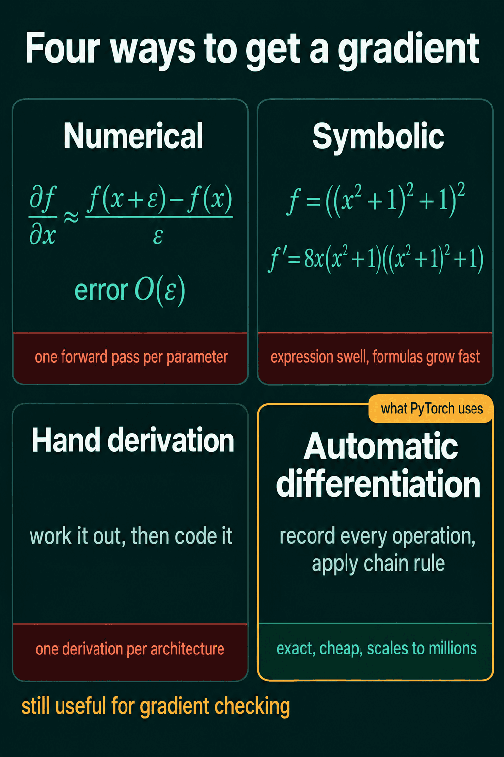
Numerical differentiation skips the calculus. It nudges one input by a small amount $\epsilon$ and measures how far the output moves:
$$\frac{\partial f}{\partial x} \approx \frac{f(x+\epsilon) - f(x)}{\epsilon}$$
Take $f(x) = x^2$ at $x = 3$, where the true derivative is $6$. With $\epsilon = 0.001$ the formula gives $(9.006001 - 9) / 0.001 = 6.001$. The error shrinks in proportion to $\epsilon$, which is written $O(\epsilon)$. Sampling both sides of $x$ is called the central difference, and it cancels the largest error term:
$$\frac{\partial f}{\partial x} \approx \frac{f(x+\epsilon) - f(x-\epsilon)}{2\epsilon}$$
The same example now gives $(9.006001 - 8.994001) / 0.002 = 6.000$, with an error that shrinks like $O(\epsilon^2)$.
1def f(x):
2    return x ** 2
3
4x, eps = 3.0, 0.001
5forward = (f(x + eps) - f(x)) / eps
6central = (f(x + eps) - f(x - eps)) / (2 * eps)
7print(forward)   # 6.000999999999479
8print(central)   # 5.999999999999339
The problem is cost. Each partial derivative needs its own extra run of the function, so a model with 50 million parameters would need 50 million runs for one gradient.
Symbolic differentiation hands the formula to software that applies the rules of calculus and returns a new formula for the derivative. The answer is exact, but the formula can grow much faster than the function. For a product of three factors $f = uvs$, the product rule gives $f' = u'vs + uv's + uvs'$, and every factor reappears in every term. Nest a few products and compositions, such as $f = ((x^2+1)^2+1)^2$ with derivative $8x(x^2+1)((x^2+1)^2+1)$, and the derivative needs more terms than the function at every level of nesting. Without careful simplification the formula gets far longer than the function it came from, which is called expression swell.
Hand derivation means working the gradient out on paper and coding it. It is exact and fast, but every new architecture needs a new derivation. A mistake in the math throws no error, so the code runs and returns wrong gradients.
Automatic differentiation records the operations your code actually executed. It then applies the chain rule numerically, one operation at a time, using values saved from the forward computation. It never builds a symbolic formula, and it scales to as many parameters as a model has.
The computation graph
The record automatic differentiation keeps is called a computation graph. Each node is one operation, and the edges show which values fed into it. When you do math on a tensor created with requires_grad=True, PyTorch computes the result and adds a node to this graph.
Take $z = 3x^2 + 1$ at $x = 2$, written as three small steps:
$$y = x^2 = 4$$
$$u = 3y = 12$$
$$z = u + 1 = 13$$
Each node stores its local gradient: how its own output changes with its own input, from basic derivative rules. The squaring node has local gradient $dy/dx = 2x$, which is $4$ at $x = 2$. The times-3 node has $du/dy = 3$. The plus-1 node has $dz/du = 1$.
Two rules cover most nodes. For an addition $z = a + b$, both local gradients are $1$, so the gradient passes through unchanged. For a multiplication $z = a \cdot b$, the local gradient for $a$ is $b$ and the local gradient for $b$ is $a$, so each input gets scaled by the other's value.
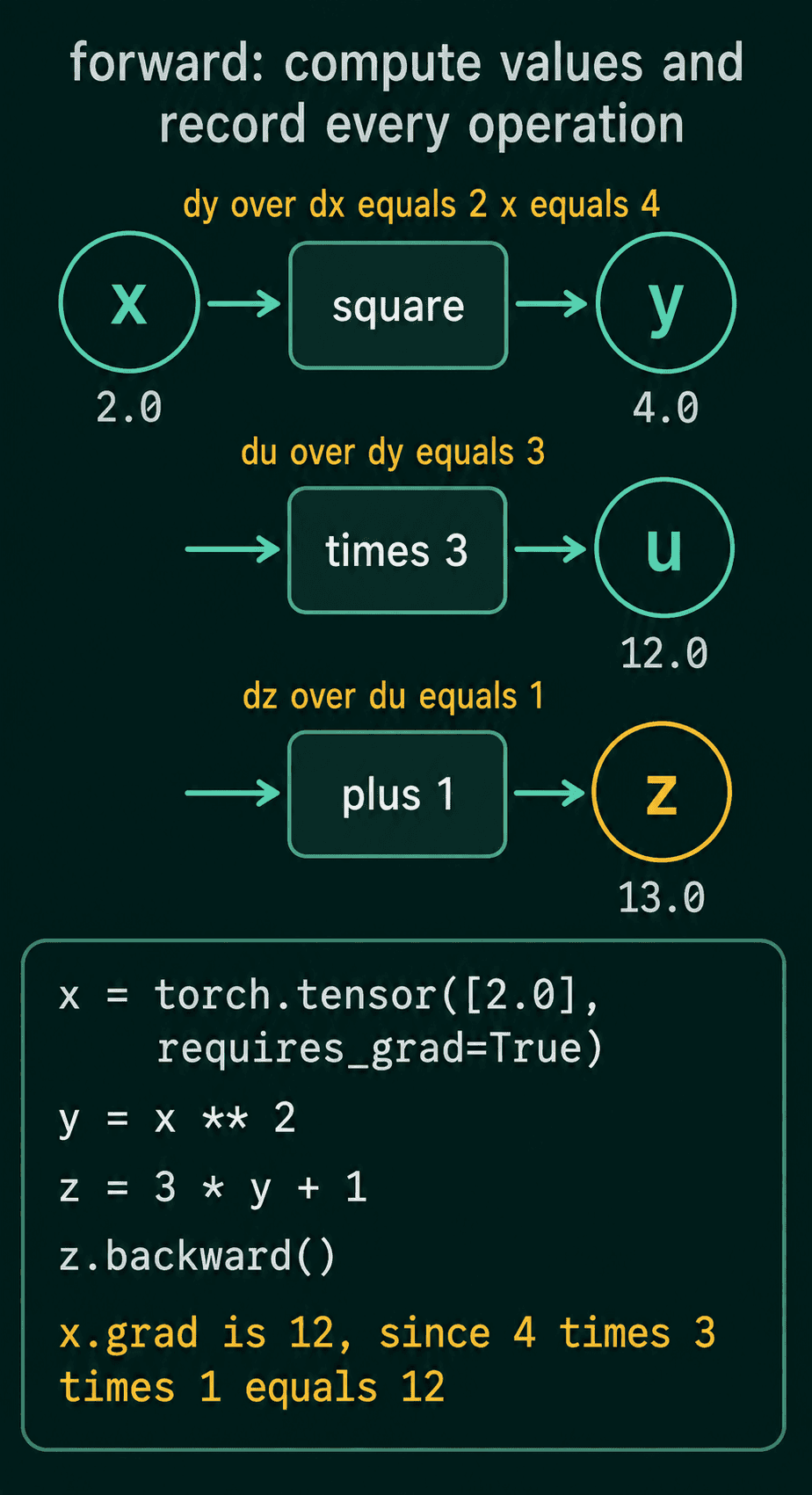
1import torch
2
3x = torch.tensor([2.0], requires_grad=True)
4y = x ** 2         # y = 4
5u = 3 * y          # u = 12
6z = u + 1          # z = 13
7
8z.backward()       # one backward sweep from z to x
9print(z)           # tensor([13.], grad_fn=<AddBackward0>)
10print(x.grad)      # tensor([12.])
The grad_fn attached to z is the graph node that produced it. That record is what .backward() walks.
Reverse mode: walking the graph backward
To get the gradient of the output for every input, PyTorch starts at the output and moves toward the inputs, multiplying local gradients along the way. In the example it starts with $dz/dz = 1$. The plus-1 node passes that through unchanged, so $dz/du = 1$. The times-3 node multiplies by 3, so $dz/dy = 3$. The squaring node multiplies by its local gradient $4$, so $dz/dx = 12$, which is the tensor([12.]) in x.grad.
Multiplying local gradients from the output back is the chain rule. Doing it automatically over a whole graph is called reverse-mode automatic differentiation. Backpropagation is reverse-mode automatic differentiation applied to a neural network's loss.
The cost is what makes it work for training. One forward pass builds the graph, and one backward sweep gives the gradient for every parameter at once. The backward sweep costs a small multiple of the forward pass. A model with 50 million parameters needs one forward pass and one backward sweep per step, where computing each partial derivative separately would need 50 million passes.
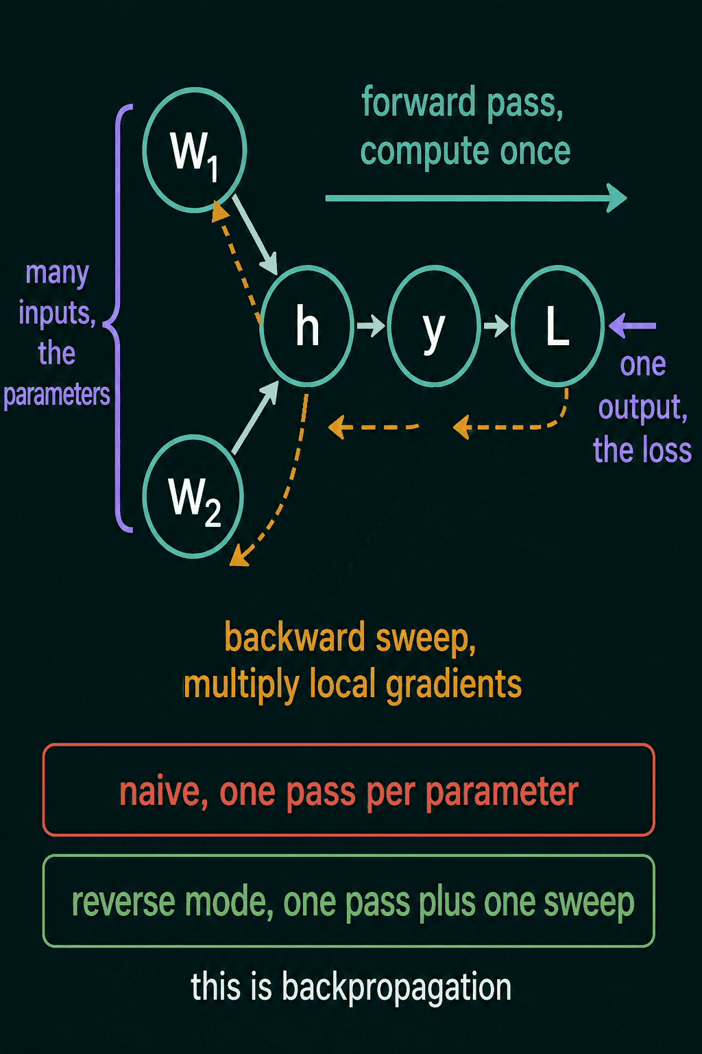
Reverse mode is cheap for one shape of computation: many inputs going into few outputs. One backward sweep gives the gradients of one output. A function with 10 outputs would need 10 sweeps. A loss has one output, so training needs one sweep.
Forward mode: carrying derivatives along
Forward-mode automatic differentiation does the opposite. It picks one input before it starts and carries a derivative next to every value as it computes forward. Alongside each value $v$ it keeps $\dot v$, the derivative of $v$ with respect to the chosen input.
On the same graph at $x = 2$, it seeds the input with $\dot x = 1$, because $dx/dx = 1$. Then $y = 4$ with $\dot y = 2x \cdot \dot x = 4$. Then $u = 12$ with $\dot u = 3 \dot y = 12$. Then $z = 13$ with $\dot z = \dot u = 12$. It reaches the same 12 in one left-to-right pass.
1# Forward mode by hand: carry (value, derivative) through every step
2x, dx = 2.0, 1.0            # seed: dx/dx = 1
3y, dy = x ** 2, 2 * x * dx  # square rule
4u, du = 3 * y, 3 * dy       # times-3 rule
5z, dz = u + 1, du           # plus-1 rule
6print(z, dz)                # 13.0 12.0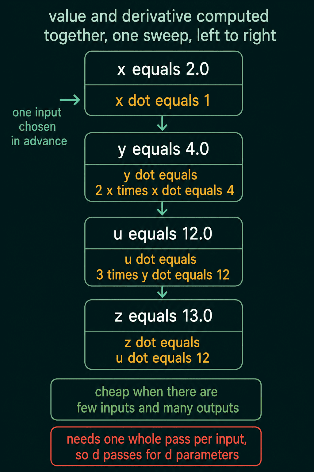
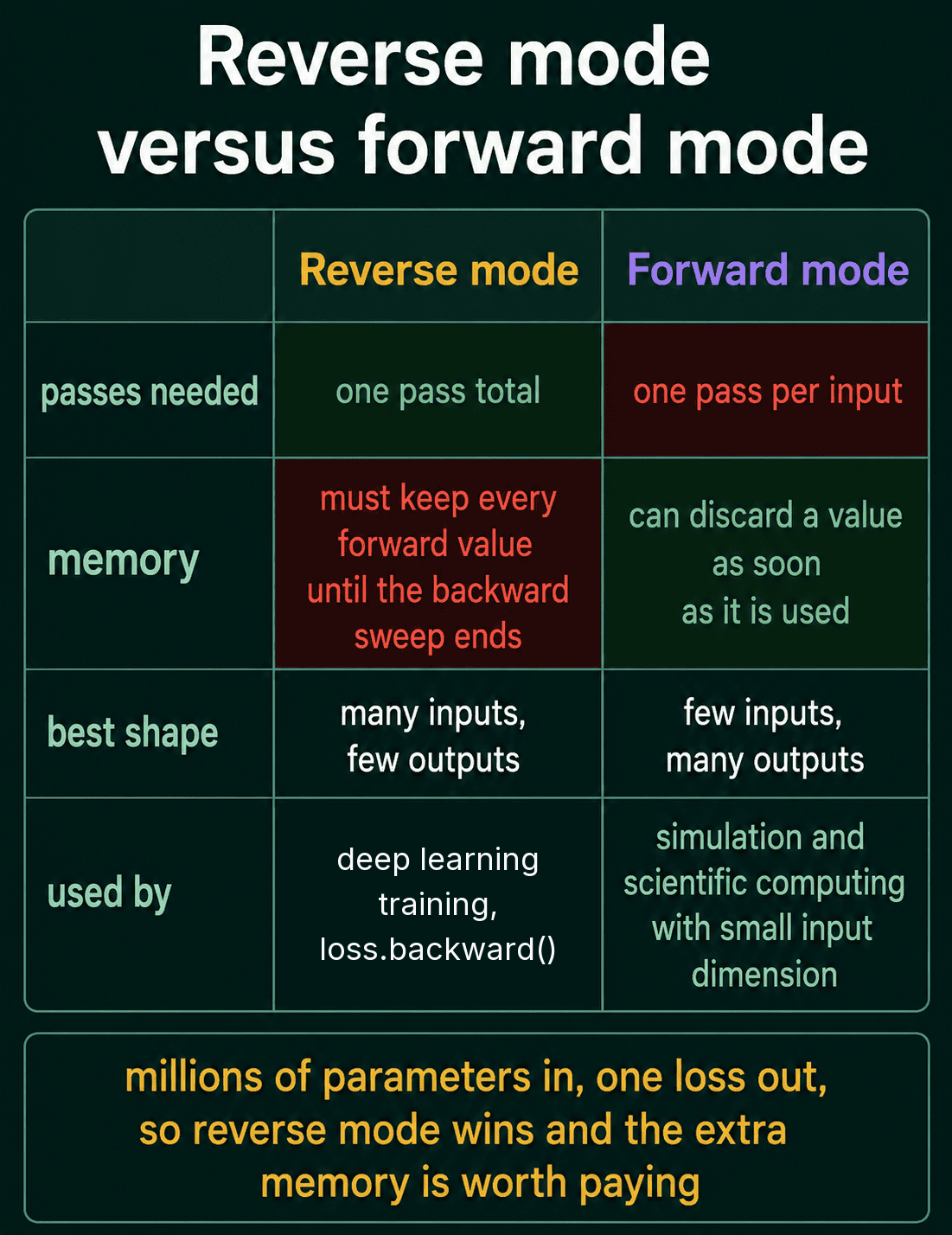
One forward-mode pass gives the derivative for one input. A gradient over $d$ parameters needs $d$ passes. Forward mode is cheap when there are few inputs and many outputs, which is the opposite of a loss function.
Why deep learning uses reverse mode
A training step has millions of inputs (the parameters) and one output (the loss). Reverse mode handles that shape with one backward sweep, and forward mode would need one pass per parameter. That is why PyTorch's .backward() is reverse mode.
Reverse mode costs memory. The backward sweep needs the intermediate values from the forward pass, so they all stay in memory until the sweep ends. Forward mode can drop each value as soon as the next step has used it. For a model with millions of parameters and one loss, the extra memory is worth it.
Checking autograd against numerical differentiation
Numerical differentiation is too slow for training, but it makes a good test. Comparing it with the gradient from your code is called gradient checking, and a mismatch points to a bug in a custom gradient. The check below uses 64-bit floats, because with 32-bit floats the rounding in the central difference is large enough to hide small bugs.
1import torch
2
3torch.manual_seed(0)
4w = torch.randn(5, dtype=torch.float64, requires_grad=True)
5x = torch.randn(5, dtype=torch.float64)
6
7def loss_fn(w):
8    return torch.sigmoid(w @ x) ** 2
9
10loss_fn(w).backward()
11autograd = w.grad.clone()
12
13# central difference, one input at a time
14eps = 1e-6
15numeric = torch.zeros(5, dtype=torch.float64)
16with torch.no_grad():
17    for i in range(5):
18        step = torch.zeros(5, dtype=torch.float64)
19        step[i] = eps
20        numeric[i] = (loss_fn(w + step) - loss_fn(w - step)) / (2 * eps)
21
22print((autograd - numeric).abs().max())   # tensor(9.1290e-14, dtype=torch.float64)
A largest difference near $10^{-13}$ means the two agree. If the difference is around $10^{-3}$ or larger, check the custom gradient code first.
When to use it, and common mistakes
You rarely call automatic differentiation directly. It runs every time you call .backward() on a loss. Knowing how it works helps when gradients come out wrong, when memory runs out during training, or when you write a custom operation.
- Forgetting that
.gradaccumulates. A second.backward()adds to the stored gradient instead of replacing it. With $x = 3$ and loss $x^2$, two calls leavex.gradat 12 instead of 6. Training loops clear it before each backward pass withoptimizer.zero_grad()orx.grad = None. - Calling
.backward()on a tensor with many values. Reverse mode starts from one output, so.backward()with no arguments expects a single number such as a summed or averaged loss. - Tracking values you only want to read. Operations on tracked tensors grow the graph and keep memory alive.
.detach()returns the same numbers cut out of the graph, which is the usual way to log a loss or store a prediction.
1import torch
2
3x = torch.tensor([3.0], requires_grad=True)
4for _ in range(2):
5    loss = (x ** 2).sum()
6    loss.backward()
7    print(x.grad)      # tensor([6.]), then tensor([12.])
8
9x.grad = None          # clear before the next backward pass
10(x ** 2).sum().backward()
11print(x.grad)          # tensor([6.])
Related concepts
The chain rule is the math each backward step applies. The Jacobian matrix generalizes a local gradient to operations with many inputs and outputs, and reverse mode multiplies by those Jacobians without building them in full. Backpropagation through a linear layer is the same backward sweep worked out by hand for $y = Wx + b$, which is a good way to see what autograd computes for the most common layer.
QuiddityML teaches automatic differentiation as its own concept in the Math track. The exercises on it include turning the central difference formula into code, spotting the bug in an autograd function and writing a gradient function with requires_grad and .backward() from scratch.