By Sagi Shaier · 13 October 2026 · 8 min read
The Hessian matrix explained, and the eigenvalue test for minima
How to compute the Hessian of a function by hand, why it is symmetric, and how its eigenvalues tell a minimum from a maximum or a saddle point, with PyTorch code to check each step.
The Hessian is the matrix of every second partial derivative of a function. Where the gradient says how steep a function is at a point, the Hessian says how that steepness is changing, which is the function's curvature. It is what separates a true minimum of a loss from a point that only looks flat.
Why the gradient is not enough
A partial derivative is the slope of a function along one input while the other inputs stay fixed. The gradient collects one partial derivative per input, so it gives the slope in every direction at once.
The slope alone leaves a gap. Take $f(x) = x^2$ and $g(x) = -x^2$ at $x = 0$. Both have slope $0$ there. But $f$ curves up and has its lowest value at $0$, while $g$ curves down and has its highest value at $0$. The difference shows up in the second derivative, the derivative of the derivative: $f''(0) = 2$ and $g''(0) = -2$. A positive second derivative means the slope is increasing, so the curve bends up. A negative one means it bends down.
For a function of several inputs there is one second derivative for every pair of inputs, and the Hessian is the matrix that holds them.
The definition
For a function $f(x, y)$ of two inputs, the Hessian $H$ is
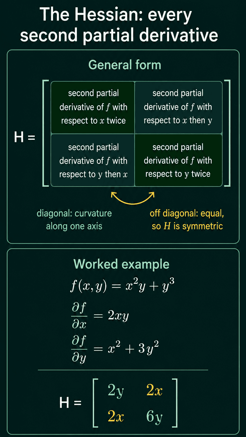
$$H = \begin{bmatrix} \dfrac{\partial^2 f}{\partial x^2} & \dfrac{\partial^2 f}{\partial x \partial y} \\[12pt] \dfrac{\partial^2 f}{\partial y \partial x} & \dfrac{\partial^2 f}{\partial y^2} \end{bmatrix}$$
Each entry means: take a partial derivative, then take another one. $\partial^2 f/\partial x^2$ differentiates with respect to $x$ twice. $\partial^2 f/\partial x \partial y$ differentiates with respect to one input, then the other.
For $n$ inputs $x_1$ through $x_n$, $H$ is an $n \times n$ matrix with one row and one column per input:
$$H_{ij} = \frac{\partial^2 f}{\partial x_i \partial x_j}$$
The diagonal entries say how the slope along one axis changes as you move along that same axis. The off-diagonal entries say how the slope along one axis changes as you move along a different axis.
A worked example
Take $f(x, y) = x^2 y + y^3$. The first partial derivatives are
$$\frac{\partial f}{\partial x} = 2xy$$
$$\frac{\partial f}{\partial y} = x^2 + 3y^2$$
Differentiate each of them again, once with respect to $x$ and once with respect to $y$. From $2xy$ you get $\partial^2 f/\partial x^2 = 2y$ and $\partial^2 f/\partial x \partial y = 2x$. From $x^2 + 3y^2$ you get $\partial^2 f/\partial y \partial x = 2x$ and $\partial^2 f/\partial y^2 = 6y$.
$$H = \begin{bmatrix} 2y & 2x \\ 2x & 6y \end{bmatrix}$$
Like the gradient, the Hessian depends on the point. At $(x, y) = (1, 2)$ it is
$$H = \begin{bmatrix} 4 & 2 \\ 2 & 12 \end{bmatrix}$$
Why the Hessian is symmetric
In the example the two off-diagonal entries came out equal: both are $2x$. That holds for any function whose second derivatives are continuous, which covers the losses used in practice. The order in which you take the two partial derivatives does not change the result, so $H_{ij} = H_{ji}$ and the Hessian is a symmetric matrix.
There is a second way to read the Hessian. The gradient takes $n$ inputs and returns $n$ numbers. The matrix of partial derivatives of any function like that is its Jacobian, so the Hessian is the Jacobian of the gradient.
1import torch
2from torch.autograd.functional import hessian
3
4def f(p):
5    x, y = p
6    return x ** 2 * y + y ** 3
7
8H = hessian(f, torch.tensor([1.0, 2.0]))
9print(H)
10# tensor([[ 4.,  2.],
11#         [ 2., 12.]])
torch.autograd.functional.hessian returns the same matrix the hand derivation gave at $(1, 2)$.
Using the Hessian at a critical point
A critical point is a point where the gradient is zero, so the function is flat in every direction. Training a model looks for low points of the loss, and low points are critical points. Not every critical point is a minimum, though. There are three kinds:
- a local minimum, where the function curves up in every direction,
- a local maximum, where it curves down in every direction,
- a saddle point, where it curves up in some directions and down in others.
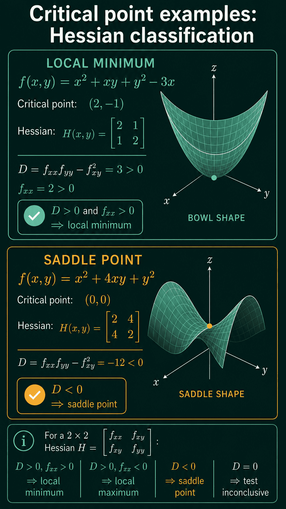
For a function of exactly two inputs there is a shortcut called the discriminant test. Compute $D = f_{xx} f_{yy} - f_{xy}^2$, where $f_{xx}$ is short for $\partial^2 f/\partial x^2$ and so on. If $D > 0$ and $f_{xx} > 0$, the point is a local minimum. If $D > 0$ and $f_{xx} < 0$, it is a local maximum. If $D < 0$, it is a saddle point, and $D = 0$ leaves it undecided.
Take $f(x, y) = x^2 + xy + y^2 - 3x$. Its gradient is $(2x + y - 3,\ x + 2y)$, which is zero at $(2, -1)$. The Hessian there is $\begin{bmatrix} 2 & 1 \\ 1 & 2 \end{bmatrix}$, so $D = 2 \cdot 2 - 1^2 = 3 > 0$ and $f_{xx} = 2 > 0$. The point is a local minimum.
Now take $f(x, y) = x^2 + 4xy + y^2$, which has a critical point at $(0, 0)$. Its Hessian is $\begin{bmatrix} 2 & 4 \\ 4 & 2 \end{bmatrix}$, so $D = 2 \cdot 2 - 4^2 = -12 < 0$. The point is a saddle.
The eigenvalue test
The discriminant only works for two inputs, and a loss can have millions. The test that scales uses the Hessian's eigenvalues.
An eigenvector of a square matrix $H$ is a direction that $H$ stretches or shrinks without turning, and its eigenvalue $\lambda$ is the stretch factor: $Hv = \lambda v$. For example, $\begin{bmatrix} 2 & 1 \\ 1 & 2 \end{bmatrix}$ maps $(1, 1)$ to $(3, 3)$, so $(1, 1)$ is an eigenvector with eigenvalue $3$. It maps $(1, -1)$ to $(1, -1)$, so that direction has eigenvalue $1$.
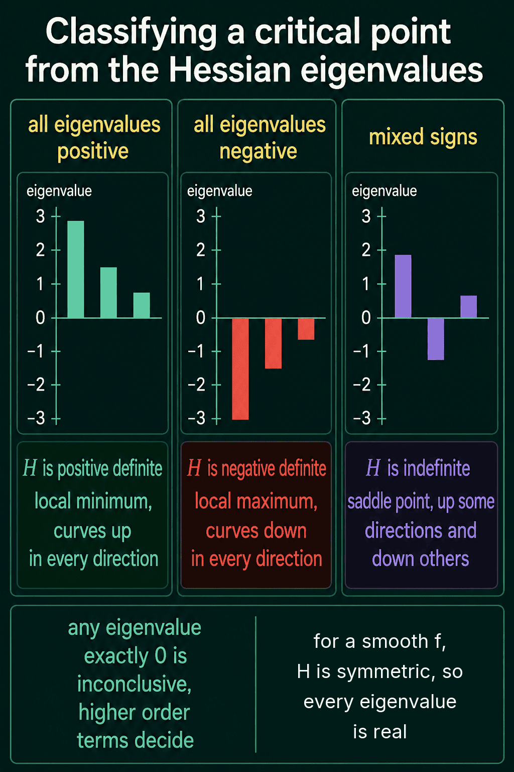
For a Hessian, each eigenvalue is the curvature of the function along its eigenvector. A positive eigenvalue means the function curves up in that direction, and a negative one means it curves down. A symmetric matrix has only real eigenvalues, so the test is well defined. At a critical point:
- All eigenvalues positive. $H$ is positive definite and the point is a local minimum.
- All eigenvalues negative. $H$ is negative definite and the point is a local maximum.
- Some positive, some negative. $H$ is indefinite and the point is a saddle.
- Any eigenvalue exactly zero. The test is inconclusive, and higher derivatives decide.
The two examples above agree with this. The bowl's Hessian has eigenvalues $1$ and $3$, both positive. The saddle's Hessian $\begin{bmatrix} 2 & 4 \\ 4 & 2 \end{bmatrix}$ has eigenvalues $6$ (along $(1, 1)$) and $-2$ (along $(1, -1)$), one of each sign. The discriminant test is the two-input version of this one: $D$ is the product of the two eigenvalues, so $D > 0$ means both have the same sign.
The test works in one direction more than the other. Positive definite at a critical point guarantees a local minimum. A local minimum does not guarantee positive definite, though. $f(x) = x^4$ has its minimum at $0$, but $f''(0) = 0$, so its Hessian there has a zero eigenvalue and the test reports inconclusive. What a local minimum does guarantee is that no eigenvalue is negative, so a single negative eigenvalue rules a point out as a minimum.
Checking eigenvalues in code
torch.linalg.eigvalsh returns the eigenvalues of a symmetric matrix, sorted from smallest to largest. The h stands for Hermitian, the complex-number version of symmetric. The test is then two comparisons on the smallest and largest eigenvalue.
1import torch
2from torch.autograd.functional import hessian
3
4def bowl(p):
5    x, y = p
6    return x ** 2 + x * y + y ** 2 - 3 * x
7
8def saddle(p):
9    x, y = p
10    return x ** 2 + 4 * x * y + y ** 2
11
12def classify(H):
13    eigs = torch.linalg.eigvalsh(H)
14    if eigs.min() > 0:
15        return eigs, "local minimum"
16    if eigs.max() < 0:
17        return eigs, "local maximum"
18    if eigs.min() < 0 < eigs.max():
19        return eigs, "saddle point"
20    return eigs, "inconclusive"
21
22print(classify(hessian(bowl, torch.tensor([2.0, -1.0]))))
23# (tensor([1., 3.]), 'local minimum')
24print(classify(hessian(saddle, torch.tensor([0.0, 0.0]))))
25# (tensor([-2.,  6.]), 'saddle point')
If a result looks wrong, check that the matrix you passed is symmetric before anything else. eigvalsh reads only the lower triangle and assumes the upper one mirrors it.
When to use it, and common mistakes
Use the Hessian to classify a critical point, to measure how curved a loss is around a point, or to check a hand derivation of second derivatives. For a full neural network, building the Hessian is rarely practical: $n$ parameters give $n^2$ entries, so a model with one million parameters would need a trillion of them.
- Calling a flat point a minimum. A zero gradient only says the point is critical. It takes the Hessian to tell a minimum from a saddle, and saddles are common in losses with many parameters.
- Treating a zero eigenvalue as a minimum. A zero eigenvalue makes the test inconclusive, as $x^4$ shows. It is not a pass.
- Passing a non-symmetric matrix to
eigvalsh. With $\begin{bmatrix} 2 & 4 \\ 0 & 2 \end{bmatrix}$, where the lower-left 4 was left out by mistake,eigvalshreads only the lower triangle and returns $2$ and $2$. The intended matrix $\begin{bmatrix} 2 & 4 \\ 4 & 2 \end{bmatrix}$ has eigenvalues $-2$ and $6$. The test would report a minimum for what is actually a saddle.
Related concepts
The Jacobian holds first derivatives of a function with several outputs, and the Hessian is the Jacobian of the gradient. Taylor series use the Hessian to add a curvature correction to the straight-line approximation of a function near a point. Convex functions are the ones whose Hessian has no negative eigenvalue anywhere, which is why any critical point of a convex function is a minimum. Positive definite matrices are the matrices whose eigenvalues are all positive, the property the minimum test checks for.
QuiddityML teaches the Hessian and the eigenvalue test as two concepts in the Math track. The exercises on them include filling in the Hessian entries for $x^2 y + y^3$, building a Hessian as a PyTorch tensor and writing an is_positive_definite check with torch.linalg.eigvalsh.