By Sagi Shaier · 14 October 2026 · 10 min read

Convex functions explained (and why neural network losses are not convex)

How to check whether a function is convex with a chord, the Hessian or a short list of known shapes, what Jensen's inequality says, and what a convex optimization problem looks like, with PyTorch code for the chord and Hessian checks.

A convex function is one whose graph never rises above the straight line drawn between any two of its points, so it is shaped like a bowl with no bumps inside it. For a convex loss, gradient descent has no false valley to settle into, because every local minimum is also a global minimum. Most deep learning losses do not have this shape, which is part of why training a neural network takes more than running the same update for longer.

Convex sets

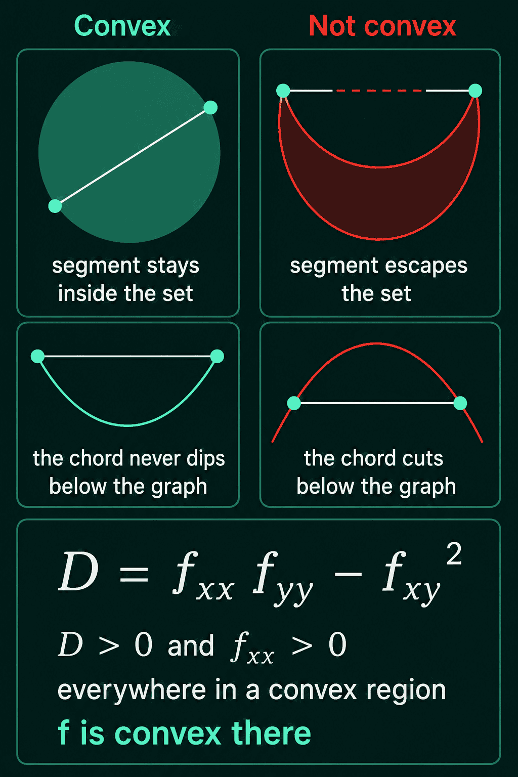
Convexity starts with sets of points. A convex set is one where the straight segment between any two points inside it stays inside it. A filled disk is convex: pick any two points in it and the segment joining them never leaves the disk. A crescent moon shape is not convex, because the segment between its two horns runs through the empty space outside the shape.

To write this down, the points on the segment between $x$ and $y$ need a formula. Every one of them is $\theta x + (1-\theta) y$ for some number $\theta$ between 0 and 1. With $\theta = 1$ the formula gives $x$, and with $\theta = 0$ it gives $y$. With $\theta = 0.5$ it gives the midpoint, so for $x = 1$ and $y = 5$ on the number line it gives $0.5 \cdot 1 + 0.5 \cdot 5 = 3$. A set $C$ is convex when

$$\theta x + (1-\theta)y \in C$$

$$\text{for all } x, y \in C \text{ and } \theta \in [0,1]$$

The symbol $\in$ means "is inside", so the condition reads: every point on the segment between two points of $C$ is also in $C$.

Convex functions

A function is convex when the same segment idea holds for its graph. Pick two inputs $x$ and $y$ and mark the points $(x, f(x))$ and $(y, f(y))$ on the graph. The straight line joining them is called a chord. The function is convex when its graph never goes above the chord:

$$f(\theta x + (1-\theta)y) \leq \theta f(x) + (1-\theta) f(y)$$

The left side is the height of the graph at a point between $x$ and $y$. The right side is the height of the chord above that same point.

Take $f(x) = x^2$ with $x = 1$, $y = 5$ and the midpoint $\theta = 0.5$. The graph at the midpoint is $f(3) = 9$. The chord there is $0.5 \cdot 1 + 0.5 \cdot 25 = 13$. Since $9 \leq 13$, the graph sits under the chord at this point, and the same holds for every pair of points on $x^2$.

Now take $f(x) = x^4 - 2x^2$, which has two low points with a bump between them. With $x = -1$ and $y = 1$ both ends sit at height $-1$, so the chord at the midpoint is $-1$. The graph at the midpoint is $f(0) = 0$. That is above the chord, so this function is not convex.

Four panels: a filled disk where the segment stays inside the set, a crescent where the segment escapes the set, a bowl-shaped curve whose chord never dips below the graph, and a hump-shaped curve whose chord cuts below the graph, above a box with the Hessian test for convexity that is explained further down

The same check takes a few lines of PyTorch. chord_gap returns the chord height minus the graph height, so a negative result means the graph poked above its chord:

1import torch
2 
3def chord_gap(f, x, y, theta):
4    """Chord height minus function height at a point between x and y."""
5    point = theta * x + (1 - theta) * y
6    chord = theta * f(x) + (1 - theta) * f(y)
7    return chord - f(point)
8 
9bowl = lambda x: x ** 2
10bump = lambda x: x ** 4 - 2 * x ** 2
11 
12x, y = torch.tensor(1.0), torch.tensor(5.0)
13print(chord_gap(bowl, x, y, 0.5))      # positive: graph under the chord
14 
15x, y = torch.tensor(-1.0), torch.tensor(1.0)
16print(chord_gap(bump, x, y, 0.5))      # negative: graph pokes above the chord
17# tensor(4.)
18# tensor(-1.)

One negative gap proves a function is not convex. Positive gaps at a few pairs do not prove it is convex, because the definition asks about every pair.

Why convexity helps gradient descent

Gradient descent moves the parameters a small step downhill at a time and stops where the slope is zero. A local minimum is a point lower than everything close to it. A global minimum is a point at least as low as every other point. On a convex function any local minimum is also a global minimum, so wherever gradient descent comes to rest there is no lower valley it missed. A convex function can still have several global minimizers at the same lowest height, but it has no false valleys.

A short run shows the difference. Gradient descent on the convex $(x-1)^2$ ends at $x = 1$ from either starting point. On the non-convex $x^4 - 2x^2 + 0.5x$, which has two valleys of different depth, the starting point decides which valley it ends in:

1import torch
2 
3def descend(f, start, lr=0.01, steps=500):
4    x = torch.tensor(start, requires_grad=True)
5    for _ in range(steps):
6        loss = f(x)
7        loss.backward()
8        with torch.no_grad():
9            x -= lr * x.grad
10        x.grad.zero_()
11    return round(x.item(), 3), round(f(x).item(), 3)
12 
13convex = lambda x: (x - 1) ** 2
14nonconvex = lambda x: x ** 4 - 2 * x ** 2 + 0.5 * x
15 
16for start in [-2.0, 2.0]:
17    print("convex   ", start, descend(convex, start))
18for start in [-2.0, 2.0]:
19    print("nonconvex", start, descend(nonconvex, start))
20# convex    -2.0 (1.0, 0.0)
21# convex    2.0 (1.0, 0.0)
22# nonconvex -2.0 (-1.057, -1.515)
23# nonconvex 2.0 (0.93, -0.517)

Starting from $x = 2$, the non-convex run stops at $x = 0.93$ with a loss of $-0.517$. That is a local minimum, while the global minimum at $x = -1.057$ has a loss of $-1.515$.

Checking convexity with the Hessian

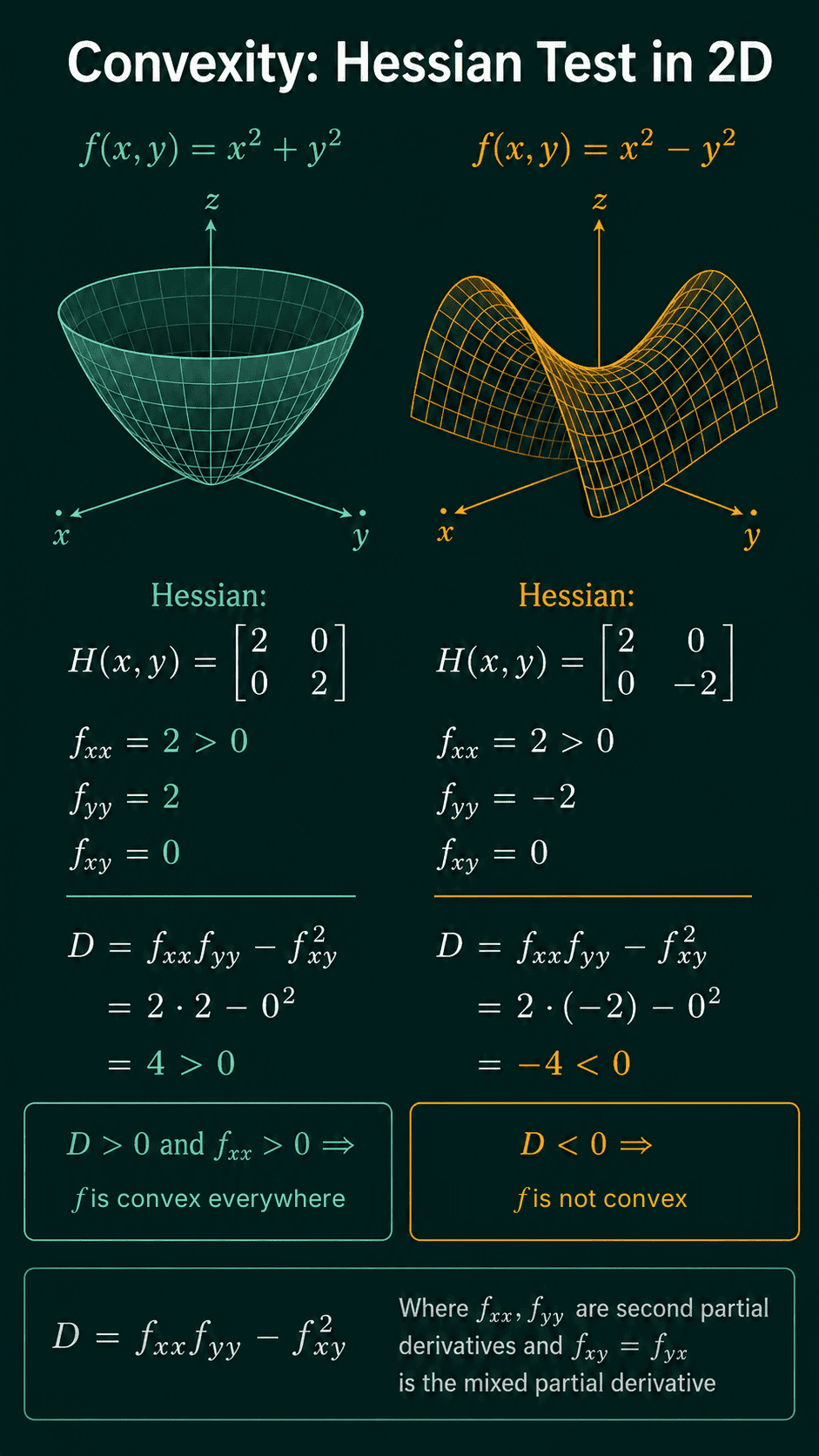
For a function of two variables, the second derivatives give a direct test. Write $f_{xx}$ for the second derivative in $x$ and $f_{yy}$ for the second derivative in $y$. The mixed one $f_{xy}$ takes one derivative in $x$ and one in $y$. Together they form the Hessian matrix:

$$H = \begin{bmatrix} f_{xx} & f_{xy} \\ f_{xy} & f_{yy} \end{bmatrix}$$

From its entries, compute the discriminant:

$$D = f_{xx} f_{yy} - f_{xy}^2$$

If $D > 0$ and $f_{xx} > 0$ at every point of a convex region, such as the whole plane, then $f$ is convex on that region. $D > 0$ says the function curves the same way in every direction, and $f_{xx} > 0$ says that way is upward.

For the bowl $f(x,y) = x^2 + y^2$, the second derivatives are $f_{xx} = 2$, $f_{yy} = 2$ and $f_{xy} = 0$. So $D = 2 \cdot 2 - 0^2 = 4 > 0$ and $f_{xx} = 2 > 0$, and the bowl is convex everywhere. The function $f(x,y) = x^2 - y^2$ curves up along $x$ and down along $y$. Its $f_{yy}$ is $-2$, which gives $D = 2 \cdot (-2) - 0^2 = -4 < 0$. The negative $D$ shows the function curves two different ways, so it is not convex.

Side-by-side 3D plots of the bowl x squared plus y squared and the saddle x squared minus y squared, each with its Hessian, second derivatives and discriminant worked out: D equals 4 for the convex bowl and D equals minus 4 for the saddle, which is not convex

A mixed term changes the numbers but not the method. For $f(x,y) = 3x^2 + 2xy + y^2$ the second derivatives are $f_{xx} = 6$, $f_{xy} = 2$ and $f_{yy} = 2$ at every point, so $D = 6 \cdot 2 - 2^2 = 8$. PyTorch can build the Hessian at a point:

1import torch
2from torch.autograd.functional import hessian
3 
4def f(p):
5    x, y = p
6    return 3 * x ** 2 + 2 * x * y + y ** 2
7 
8H = hessian(f, torch.tensor([0.5, -2.0]))
9f_xx, f_xy, f_yy = H[0, 0], H[0, 1], H[1, 1]
10D = f_xx * f_yy - f_xy ** 2
11print(H)
12print(D, f_xx)    # D > 0 and f_xx > 0: convex
13# tensor([[6., 2.],
14#         [2., 2.]])
15# tensor(8.) tensor(6.)

The point $(0.5, -2)$ is arbitrary, since a quadratic like this one has the same Hessian everywhere. If hessian raises an error, check that f returns a single number and not a vector.

Convex functions you can recognize on sight

The Hessian test is one way to check convexity. A short list of known shapes often answers the question faster:

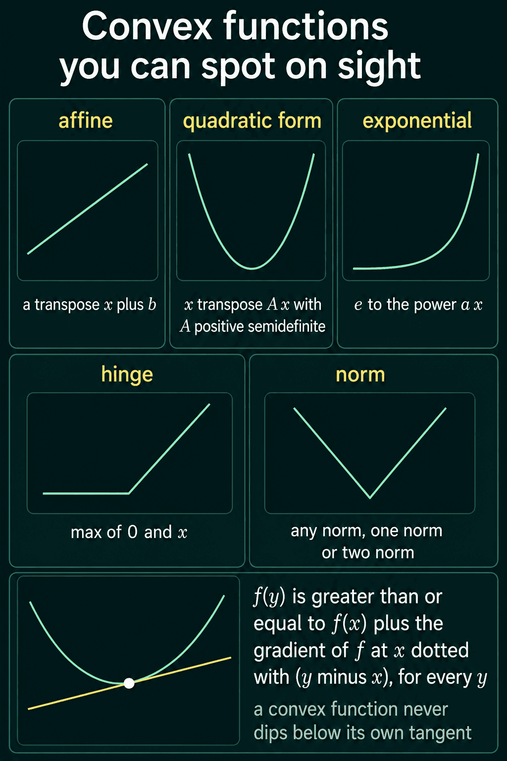
Affine functions $a^T x + b$, which are straight lines and flat planes.
Quadratic forms $x^T A x$ where $A$ is positive semidefinite, meaning $x^T A x \geq 0$ for every $x$. With $A$ the identity matrix this is $\|x\|_2^2$, the sum of squared entries.
The exponential $e^{ax}$ for any number $a$.
The hinge $\max(0, x)$, which is the shape of the ReLU activation and of the hinge loss $\max(0, 1 - y f(x))$ used by support vector machines (SVMs).
Every norm, such as $\|x\|_1$ (the sum of absolute values) or $\|x\|_2$ (the length), even though a norm has a sharp corner at the origin.
$-\log x$ for $x > 0$. The logarithm curves downward, which makes it concave, and flipping its sign gives a convex function. That is why $-\log$ turns up in loss functions.

There is also a test that uses only the first derivative. At any point $x$, the tangent is the straight line (or flat plane) that touches the graph at $x$ with the same slope. For a convex function, the tangent at any point lies at or below the graph everywhere:

$$f(y) \geq f(x) + \nabla f(x)^T (y-x)$$

Here $\nabla f(x)$ is the gradient, the vector of slopes at $x$, and the right side is the height of the tangent above $y$. For $f(x) = x^2$ at $x = 1$ the tangent is $1 + 2(y - 1)$. At $y = 4$ the tangent gives $7$ and the graph gives $f(4) = 16$, so the graph is above the tangent there.

Five small plots of convex building blocks: an affine line, a quadratic form bowl, an exponential curve, the hinge max of 0 and x, and the V shape of a norm, above a curve with its tangent line touching it from below and the first-order condition written out

Jensen's inequality

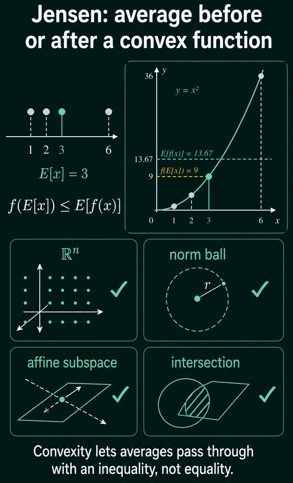
Convex functions come with one useful inequality. The expected value $E[x]$ is the average of $x$, weighted by how often each value occurs. If $x$ is equally likely to be $1$, $2$ or $6$, then

$$E[x] = \frac{1+2+6}{3} = 3$$

$$E[x^2] = \frac{1+4+36}{3} = \frac{41}{3} \approx 13.67$$

Squaring the average gives $3^2 = 9$, while averaging the squares gives $13.67$. Jensen's inequality says that for a convex $f$ the first is never larger than the second:

$$f(E[x]) \leq E[f(x)]$$

ML derivations use it to move an average across a nonlinear function, often to turn a quantity that cannot be computed into a bound that can.

Convex sets have a short list too. The whole space $\mathbb{R}^n$ is convex, and so is any ball defined by a norm. Any line or plane is convex, including one shifted away from the origin (an affine subspace). The overlap of any number of convex sets is convex, and so is the set of all positive semidefinite matrices of a given size.

The values 1, 2 and 6 on a number line with their average 3, next to the curve y equals x squared where squaring the average gives 9 and averaging the squares gives 13.67, above four convex sets: all of R n, a norm ball, an affine subspace and the intersection of two convex sets

What a convex optimization problem looks like

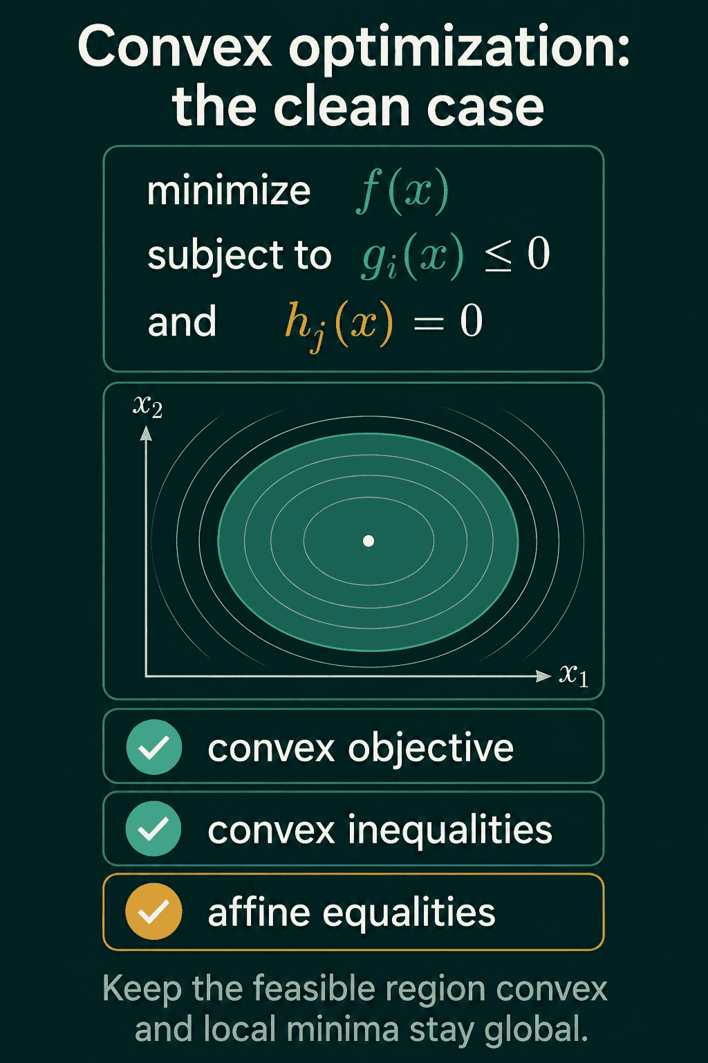
Some problems come with constraints, such as weights that have to stay non-negative. A convex optimization problem has this form:

$$\text{minimize } f(x)$$

$$\text{subject to } g_i(x) \leq 0, \quad i = 1, \dots, m$$

$$h_j(x) = 0, \quad j = 1, \dots, p$$

Here $f$ and every $g_i$ are convex, and every $h_j$ is affine, meaning a linear function plus a constant. Those conditions keep the set of allowed points convex, so any local minimum of the constrained problem is still a global minimum. Break one of them and the guarantee can fail.

The convex optimization form, minimize f of x subject to convex inequality constraints and affine equality constraints, above a contour plot of a convex bowl with its single minimum and three checks: convex objective, convex inequalities, affine equalities

Why neural network losses are not convex

A neural network's loss, viewed as a function of its weights, is usually not convex. It has local dips, flat stretches and points where the slope is zero without being a minimum. The guarantee from the convex case does not carry over, so where gradient descent ends up depends on where it starts and how it moves, as the $x^4 - 2x^2 + 0.5x$ run showed. Losses built from the shapes above keep the guarantee, such as a squared error on a linear model or the SVM hinge loss, which is why many classical ML problems reach their best answer.

When to use it, and common mistakes

Check convexity when you pick or design a loss for a classical model, or when a derivation needs Jensen's inequality. For a deep network the answer is usually "not convex", so the useful question becomes how the optimizer copes with that.

Testing at one point only. The Hessian test has to pass everywhere on the region. For $x^4 - 2x^2$ the second derivative $12x^2 - 4$ is $8$ at $x = 1$ and $-4$ at $x = 0$, so a check at $x = 1$ alone would miss the bump.
Reading $D > 0$ alone as convex. $D > 0$ with $f_{xx} < 0$ means the function curves downward in every direction, which is concave. $-x^2 - y^2$ gives $D = 4$ and $f_{xx} = -2$.
Reading an inconclusive test as a no. The Hessian test is sufficient, not necessary. $x^4 + y^4$ is convex, but at the origin every second derivative is 0, so $D = 0$ and the test says nothing there.
Mixing up convex and concave. $\log x$ is concave and $-\log x$ is convex.

The Hessian is the matrix of second derivatives that the convexity test reads. Critical points are where the gradient is zero, and on a non-convex loss they include local minima, local maxima and saddle points. Positive semidefinite matrices are the matrices whose quadratic form is never negative, and a twice-differentiable function is convex exactly when its Hessian is positive semidefinite everywhere.

QuiddityML teaches convex functions and convex sets as their own concept in the Math track. The exercises on it include applying the discriminant test to a Hessian, ordering the lines of a passes_convexity_test function and then writing that function from scratch.