By Sagi Shaier · 6 October 2026 · 6 min read

ML model monitoring after deployment: data drift and when to retrain

A model that tested well can get worse after launch because the data it sees keeps changing while the model stays the same. This post explains how that happens, how to notice it, and how to retrain and replace a live model safely in PyTorch.

Model monitoring is checking how a deployed model performs on the data it receives after launch, so you find out when its predictions start getting worse. They often do, even when no one has touched the code, because the data the model sees keeps changing while the model's weights stay frozen at whatever training produced. That change is usually called data drift, and the usual response to it is a loop of monitoring, retraining, and carefully swapping in the new model.

How a trained model gets used after launch

A trained model on its own makes no predictions until some other code calls it. The simplest setup loads the model inside the application and calls it directly: model.eval() switches layers like dropout to inference behavior, and torch.no_grad() tells PyTorch not to track gradients, since nothing is being trained. That works for a small project, but it ties the model to the code that calls it, so upgrading the model means editing that code too.

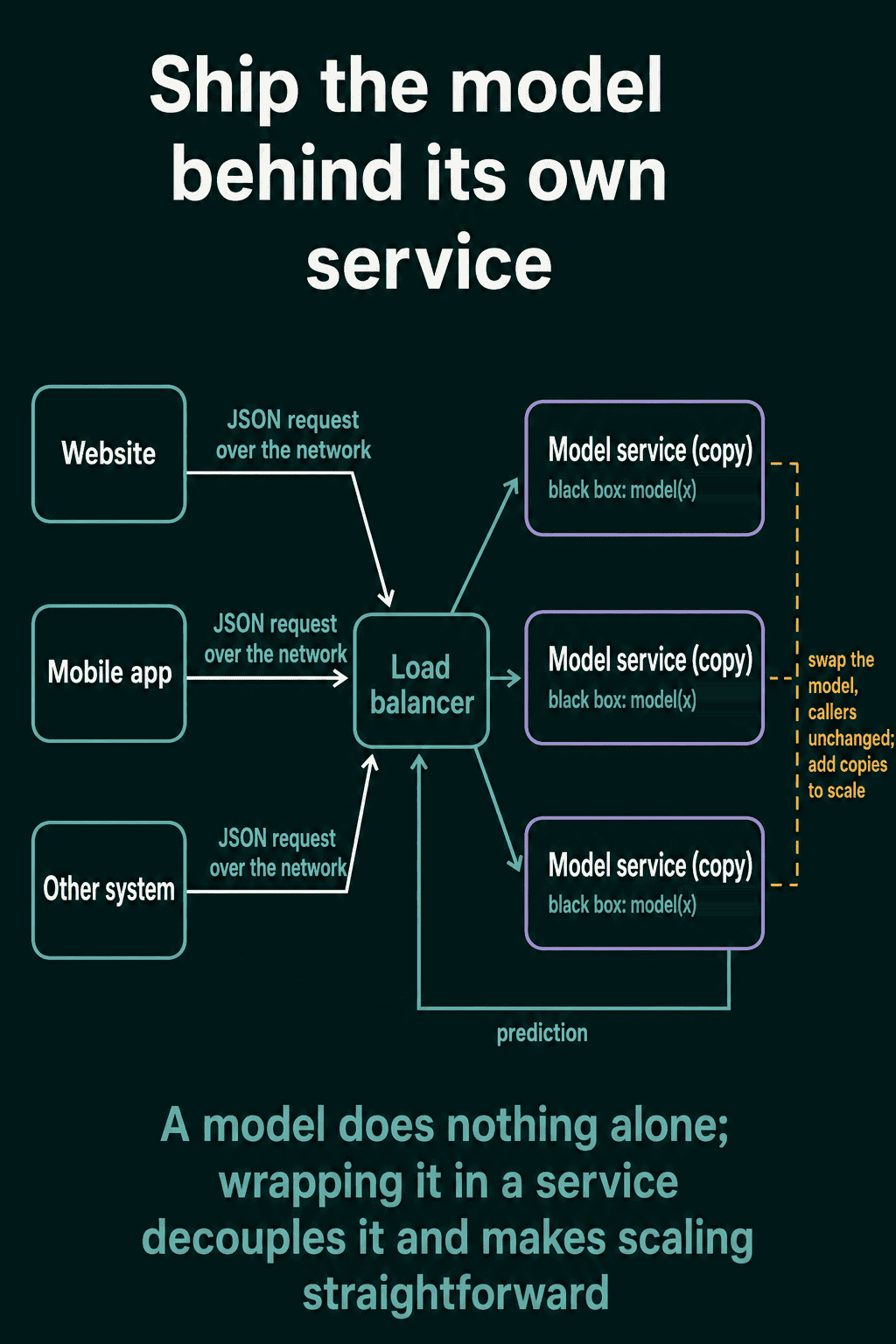
A more common setup after launch puts the model behind its own small service: a program that receives input over the network, usually as JSON, runs the model, and sends the prediction back. A website, a mobile app, or any other system calls that service without knowing what model is inside. If traffic grows, you run more copies of the service behind a load balancer, which spreads incoming requests across the copies.

A website, a mobile app, and another system sending JSON requests over the network to a load balancer that spreads them across three copies of a model service, each a black box running model(x), with predictions sent back

The running example in this post is a small fraud detector. Each transaction has two features: a spending amount and a second signal. The model is trained on one period's transactions and labels a transaction as fraud when it looks unusual for the prices of that period:

1import torch
2import torch.nn as nn
3 
4torch.manual_seed(0)
5 
6def make_data(n, shift=0.0):
7    # Two features per transaction: spending amount and a second signal.
8    x = torch.randn(n, 2)
9    x[:, 0] += shift                                 # a pricing change moves every amount
10    y = (x[:, 0] - shift + 0.5 * x[:, 1] > 1.0).float()   # fraud = unusual for the current prices
11    return x, y
12 
13def train(x, y, steps=500):
14    model = nn.Sequential(nn.Linear(2, 16), nn.ReLU(), nn.Linear(16, 1))
15    opt = torch.optim.Adam(model.parameters(), lr=0.01)
16    loss_fn = nn.BCEWithLogitsLoss()
17    for _ in range(steps):
18        opt.zero_grad()
19        loss = loss_fn(model(x).squeeze(1), y)
20        loss.backward()
21        opt.step()
22    return model
23 
24def accuracy(model, x, y):
25    model.eval()
26    with torch.no_grad():
27        preds = (model(x).squeeze(1) > 0).float()
28    return (preds == y).float().mean().item()
29 
30x_old, y_old = make_data(2000)
31live_model = train(x_old, y_old)
32x_test, y_test = make_data(500)
33print(f"accuracy at launch: {accuracy(live_model, x_test, y_test):.3f}")   # 0.998

The function a service would run on each request looks like this. It takes the features from the request, runs the model without gradients, and returns a JSON-ready answer:

1def predict(model, features):
2    model.eval()
3    with torch.no_grad():
4        logit = model(torch.tensor([features]))
5    return {"fraud": bool(logit.item() > 0)}
6 
7print(predict(live_model, [0.2, -0.4]))   # {'fraud': False}
8print(predict(live_model, [2.5, 1.0]))    # {'fraud': True}

Why models go stale after deployment

After training, the model's weights stay fixed, and the world it makes predictions about keeps moving. Customer behavior changes, a sensor gets replaced with a different one, trends come and go. Each of these shifts the data arriving at the model away from the data it was trained on, and a model left alone slowly falls out of step with what it now sees. This gradual loss of accuracy is sometimes called model rot, and it can happen with no bugs in the code at all.

The fraud detector shows it directly. Suppose a pricing change raises every spending amount. What counts as normal spending has moved, but the model's idea of suspicious spending is still tuned to the old prices, so it starts flagging ordinary purchases. In the code, shift is how far the amounts have moved, and the labels follow the new prices.

How to notice a model getting worse

Sometimes you notice it indirectly, through a number the business already tracks, such as sales dropping or click-through rate falling. When no number like that exists, the usual fallback is human review: on a schedule, people label a sample of the model's recent predictions, and you measure accuracy on that sample.

Here is that review run over four months, with amounts moving further each month:

1for month, shift in enumerate([0.0, 0.5, 1.0, 1.5], start=1):
2    x_month, y_month = make_data(200, shift=shift)   # a reviewed sample of 200 predictions
3    print(f"month {month}: accuracy {accuracy(live_model, x_month, y_month):.3f}")

1month 1: accuracy 0.995
2month 2: accuracy 0.925
3month 3: accuracy 0.620
4month 4: accuracy 0.505

The model and its code are the same in all four months. Only the data changed, and accuracy went from 0.995 to 0.505, which for a yes-or-no fraud call is close to a coin flip.

When and how to retrain

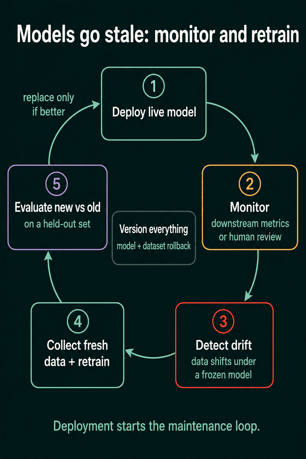
A one-time retrain fixes this month and leaves the model to drift again. The usual fix is a loop that runs on a schedule:

Collect fresh labeled data from the period the model is now serving.
Retrain a new candidate model on it.
Evaluate the candidate and the live model on the same held-out set, recent data that neither model trained on.
Replace the live model only if the candidate scores better.

The comparison in step 3 is there because a retrained model is not guaranteed to be better. If the fresh data is corrupted or does not represent real traffic, retraining can make the model worse, and promoting it without a check would replace a working model with a broken one. Doing this by hand gets slow as the number of models grows, so it is worth automating as much of the loop as you can.

1x_fresh, y_fresh = make_data(2000, shift=1.5)        # fresh labeled data
2x_held, y_held = make_data(500, shift=1.5)           # held-out set from the same period
3candidate = train(x_fresh, y_fresh)
4 
5old_acc = accuracy(live_model, x_held, y_held)
6new_acc = accuracy(candidate, x_held, y_held)
7print(f"live model: {old_acc:.3f}  candidate: {new_acc:.3f}")   # live model: 0.546  candidate: 1.000
8 
9torch.save(live_model.state_dict(), "model_v1.pt")   # keep the old version on disk
10if new_acc > old_acc:
11    torch.save(candidate.state_dict(), "model_v2.pt")
12    live_model = candidate
13    print("promoted model_v2")

On the held-out set from the shifted period, the live model scores 0.546 and the candidate scores 1.000, so the candidate is promoted. The candidate's perfect score comes from the toy data, where the fraud rule is exact. On real data, expect a smaller gap.

Versioning models and datasets

The code above saves the old model to model_v1.pt before promoting the new one. Keeping each model version, and the dataset version it was trained on, means a bad deploy is a quick rollback instead of a rebuild. If a freshly promoted model starts misbehaving, you load the previous weights and put them back in service:

1rollback = nn.Sequential(nn.Linear(2, 16), nn.ReLU(), nn.Linear(16, 1))
2rollback.load_state_dict(torch.load("model_v1.pt"))
3print(f"restored v1, held-out accuracy {accuracy(rollback, x_held, y_held):.3f}")   # 0.546

The restored model gives the same 0.546 as before, which confirms the saved weights are the ones that were live. The full loop, from deploying to monitoring to retraining and back, with versioning underneath it:

A five-step loop: 1 deploy live model, 2 monitor through downstream metrics or human review, 3 detect drift as data shifts under a frozen model, 4 collect fresh data and retrain, 5 evaluate new vs old on a held-out set, with an arrow back to deploy labeled replace only if better and a center box reading version everything, model plus dataset rollback

Common mistakes

Treating launch as the end. A model with good test scores can lose accuracy on shifting data, and without monitoring the drop can go unnoticed until a downstream number falls.
Promoting every retrained model. Without a held-out comparison against the live model, a retrain on bad data goes straight to users.
Comparing on different data. The live model and the candidate need to be scored on the same held-out set, or the comparison says nothing about which one to keep.
Overwriting the old weights. Saving the new model over the old file removes the rollback. Keep each version.
Calling the model without model.eval() and torch.no_grad(). In serving code, dropout and batch normalization behave differently in training mode, and tracking gradients wastes memory on every request.

The held-out set used to compare models follows the same rules as a test set during development, covered in train, validation, and test sets. Which number to compare the two models on depends on the task, and how to choose an evaluation metric goes through the options. A served model also has to answer fast enough, and how to measure model size and speed covers latency and throughput. Saving and loading state_dict files is the same mechanism used for training checkpoints in how to save and resume training in PyTorch.

QuiddityML teaches deployment and model staleness as the Launch, Monitor, and Maintain concept in the ML Foundation track, and the exercises on it ask why a model behind a service is easier to upgrade, why accuracy drops after launch with no code change, and how to decide whether a retrained model should replace the live one.