By Sagi Shaier · 6 October 2026 · 7 min read

A step-by-step workflow for improving a machine learning model

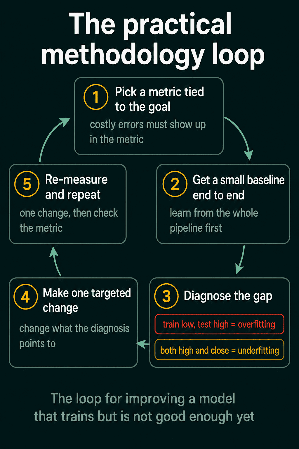
When a model trains but its results are not good enough, a five-step loop tells you what to change next: pick a metric tied to the goal, build a small baseline, read the gap between training and test error, make one targeted change, and measure again.

A machine learning workflow is the loop you repeat to take a model that trains without errors and make it good enough for the job it was built for. Most of the time spent on a real project goes into this loop, and the usual way it goes wrong is guessing: trying a bigger model, then a new feature, then a different optimizer, with no way to tell which change helped. The workflow below has five steps: pick a metric tied to the goal, get a small baseline working end to end, diagnose the gap between training and test error, make one targeted change, and re-measure.

A broken model and a weak model need different tools

A training run can fail in two different ways. In the first, something is broken: the loss turns into NaN, or it stays flat from the first step. That calls for low-level debugging, such as checking where the NaN appears, training on a single batch to confirm the model can fit it, and looking at gradient sizes per layer. Loss is NaN: the common causes and fixes and the loss-not-decreasing checklist cover that case.

In the second, training works, the loss goes down, and the model still makes too many mistakes on the data you care about. Nothing is broken, so a debugging checklist has nothing to find. This post is about that second case, the layer above debugging.

Step 1: Pick a metric tied to the goal

A metric is the number you use to decide whether the model got better. The usual default is accuracy, the fraction of predictions that are correct, or its mirror image, the error rate. The problem is that accuracy counts every mistake the same, and real goals rarely do.

Take a model that flags a rare disease. A false negative is a sick patient the model calls healthy, and a false positive is a healthy patient it flags. If false negatives are expensive, that cost has to show up in the metric you optimize. Here that means tracking recall, the fraction of real positives the model catches, next to the error rate, and judging each change by whether recall moved. A note saying "watch the false negatives" written next to an accuracy number does not do that job, because each decision still gets made by looking at accuracy.

How to turn the cost of each kind of mistake into a choice of metric gets its own post in how to choose an evaluation metric.

Step 2: Get a small baseline working end to end

A baseline is the simplest model you can build that runs through the whole pipeline: load the data, train, predict, and compute the metric from Step 1. A rough version of the whole pipeline teaches you more than a polished version of one piece, because it shows where the real problem is before you spend a week on a part that turns out to be fine.

The script below is a small classification problem. Each point has two features, and its label is 1 when the point falls inside a circle and 0 otherwise. The report function prints the error rate and the recall on the training data and on a separate test set the model never trains on:

1import torch
2import torch.nn as nn
3 
4torch.manual_seed(0)
5 
6def make_data(n):
7    x = torch.randn(n, 2)
8    y = (x.pow(2).sum(dim=1) < 0.7).float()   # 1 inside a circle, 0 outside
9    return x, y
10 
11x_train, y_train = make_data(2000)
12x_test, y_test = make_data(2000)
13print(f"positives in train: {y_train.mean().item():.0%}")   # positives in train: 31%
14 
15def train(model, x, y, epochs=500, weight_decay=0.0):
16    opt = torch.optim.Adam(model.parameters(), lr=0.01, weight_decay=weight_decay)
17    loss_fn = nn.BCEWithLogitsLoss()
18    for _ in range(epochs):
19        opt.zero_grad()
20        loss = loss_fn(model(x).squeeze(1), y)
21        loss.backward()
22        opt.step()
23    return model
24 
25@torch.no_grad()
26def report(name, model, x_tr, y_tr):
27    for split, x, y in [("train", x_tr, y_tr), ("test", x_test, y_test)]:
28        pred = (model(x).squeeze(1) > 0).float()
29        error = (pred != y).float().mean().item()
30        recall = (pred[y == 1] == 1).float().mean().item()
31        print(f"{name:<9} {split:<5} error {error:.3f}  recall {recall:.3f}")

The baseline is a single linear layer, which can only draw a straight line between the two classes:

1baseline = train(nn.Linear(2, 1), x_train, y_train)
2report("baseline", baseline, x_train, y_train)

1baseline  train error 0.312  recall 0.000
2baseline  test  error 0.287  recall 0.000

An error rate of 0.287 means about 71% accuracy, which can look acceptable at a glance. The recall of 0 shows what is really going on: the model labels every point 0 and catches none of the positives, and since 31% of the training points are positive, that alone gives the 0.312 training error. This is Step 1 paying off, because accuracy alone would have hidden it.

Step 3: Diagnose the gap

Training error is the error on the data the model was trained on, and test error is the error on held-out data it never saw. Comparing the two tells you what kind of problem you have:

Training and test error close together and both too high: the model is underfitting. It cannot fit even the data it trains on, so it is too simple for the problem or missing information it needs.
Training error low but test error high: the model is overfitting. It fits the training data, including details that do not carry over to new data, and does worse on data it has not seen.

The baseline has a training error of 0.312 and a test error of 0.287: close together and both far too high, so it is underfitting. That rules out a whole group of fixes before trying any of them, since adding more data or more regularization targets overfitting and would not help a straight line fit a circle. Overfitting vs underfitting goes deeper into reading the two from loss curves.

Step 4: Make one targeted change and re-measure

The usual changes are a bigger model, more data, better features, or a different amount of regularization (anything that limits how closely the model can fit the training data, such as weight decay, which pulls the weights toward zero). Each one targets one side of the diagnosis:

Diagnosis	Changes that match it
Underfitting	bigger model, better features
Overfitting	more data, more regularization

Make one change at a time and run the same report after it. If you change the model size and the features together and the test error drops, you do not know which change did it, or whether one helped while the other hurt.

For the underfitting baseline, the matching change is a bigger model. Adding one hidden layer of 32 units with a ReLU between them lets the model draw a curved boundary:

1torch.manual_seed(0)
2bigger = train(nn.Sequential(nn.Linear(2, 32), nn.ReLU(), nn.Linear(32, 1)), x_train, y_train)
3report("bigger", bigger, x_train, y_train)

1bigger    train error 0.004  recall 0.994
2bigger    test  error 0.004  recall 0.995

Test error fell from 0.287 to 0.004 and test recall rose from 0 to 0.995, and the train and test numbers are still close together, so the change fixed the underfitting without causing overfitting.

To see what overfitting looks like in the same report, the run below trains a much larger network on only the first 50 training points:

1torch.manual_seed(0)
2x_small, y_small = x_train[:50], y_train[:50]
3big = nn.Sequential(nn.Linear(2, 256), nn.ReLU(), nn.Linear(256, 256), nn.ReLU(), nn.Linear(256, 1))
4overfit = train(big, x_small, y_small, epochs=2000)
5report("50 rows", overfit, x_small, y_small)

150 rows   train error 0.000  recall 1.000
250 rows   test  error 0.062  recall 0.941

Training error is 0 and test error is 0.062, so the model is overfitting. A bigger model would make this worse. The matching change is more data, so the same network now trains on all 2000 points:

1torch.manual_seed(0)
2big = nn.Sequential(nn.Linear(2, 256), nn.ReLU(), nn.Linear(256, 256), nn.ReLU(), nn.Linear(256, 1))
3more_data = train(big, x_train, y_train, epochs=2000)
4report("2000 rows", more_data, x_train, y_train)

12000 rows train error 0.000  recall 1.000
22000 rows test  error 0.002  recall 0.998

Test error dropped from 0.062 to 0.002. When more data is not available, the weight_decay argument in train is the other change that targets overfitting. If a change does not move the metric, undo it, go back to Step 3, and check the diagnosis again before trying the next one.

Step 5: Repeat

After each change, the numbers from Step 4 become the new starting point. Diagnose the gap again, because a fix for underfitting can push a model into overfitting, and the next change has to match the new diagnosis. The loop stops when the metric from Step 1 is good enough for the goal, which is why that metric has to be the one the goal depends on.

The practical methodology loop as five connected boxes: 1 pick a metric tied to the goal, 2 get a small baseline end to end, 3 diagnose the gap with train low and test high meaning overfitting and both high and close meaning underfitting, 4 make one targeted change, 5 re-measure and repeat, then back to 1

Common mistakes

Changing several things at once. The metric moves and nothing tells you which change moved it.
Picking a fix before the diagnosis. More data does little for an underfitting model, and a bigger model usually makes overfitting worse.
Optimizing accuracy when one kind of mistake costs more. The baseline above reached about 71% accuracy while catching zero positives.
Polishing one stage before the pipeline runs end to end. Weeks spent on features can turn out to be wasted if the real problem is in the labels or the evaluation.

The low-level debugging checks for a run that is broken are in the loss-not-decreasing checklist. Measuring each change on the same held-out set many times can make that number look better than the model really is, and data leakage in machine learning explains why and how a separate validation set helps. Regularization, the main change for overfitting when more data is not an option, is covered in regularization explained.

QuiddityML teaches this loop as the Practical Methodology concept in the ML Foundation track, and its exercises ask how it differs from low-level debugging of a broken run and what to check first when a working model is not good enough.