By Sagi Shaier · 6 October 2026 · 8 min read

How to measure model size and speed: parameters, FLOPs, latency, throughput, memory

Accuracy says how good a model's predictions are, not whether it is small and fast enough to run. This post shows how to measure parameter count, FLOPs, latency, throughput, and memory in PyTorch, and which one to look at for which job.

Model efficiency is how much a model costs to store and run: how many numbers it holds, how much arithmetic one prediction takes, how long a user waits for an answer, how many answers it gives per second, and how much memory it fills. Accuracy says nothing about any of these, and a model too slow or too large for its device is of little use however well it scores.

Why accuracy alone is not enough

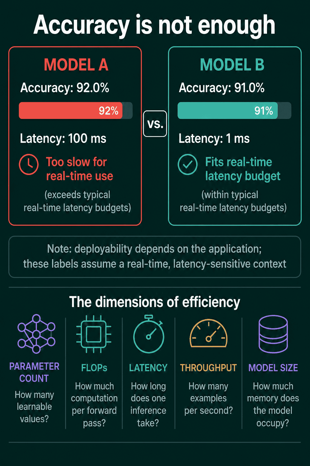
Take two models for a real-time feature such as autocomplete. Model A reaches 92% accuracy and takes 100 ms per prediction. Model B reaches 91% and takes 1 ms. A real-time app has a latency budget, the longest it can wait for a prediction before the user notices, and 100 ms is past the typical budget for this kind of feature. Model B is the one to ship here, a point lower and 100 times faster.

Efficiency is measured along five dimensions:

Parameter count: how many learnable values the model has.
FLOPs: how much arithmetic one forward pass takes.
Latency: how long one prediction takes.
Throughput: how many examples the model handles per second.
Model size: how much memory the model occupies.

Model A at 92% accuracy and 100 ms marked too slow for real-time use, Model B at 91% and 1 ms marked within budget, and the five dimensions of efficiency

Parameter count

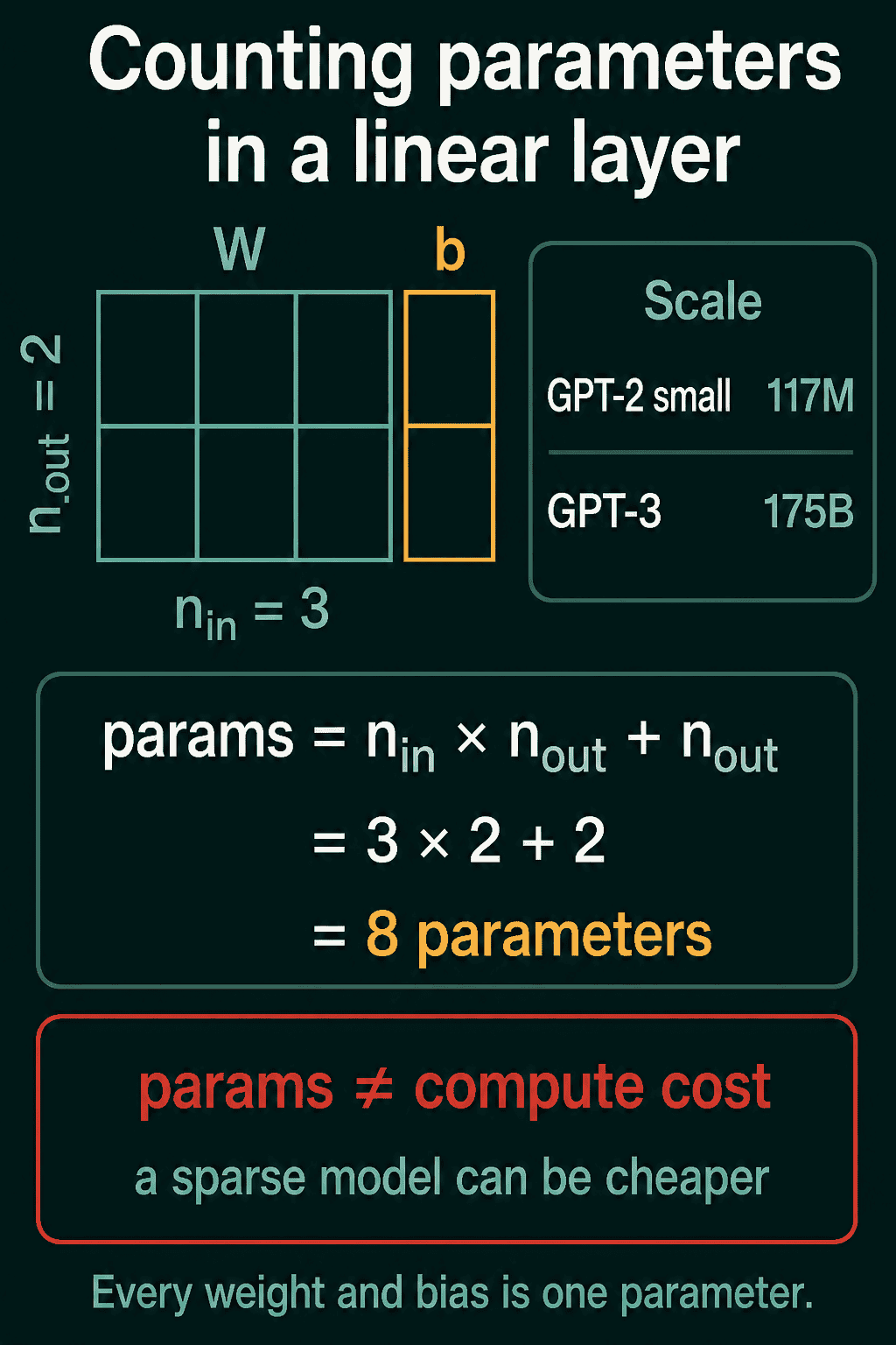
A parameter is one learnable number in the model, a weight or a bias that training adjusts. A linear layer with $n_{\text{in}}$ inputs and $n_{\text{out}}$ outputs has a weight matrix $W$ with one weight per input-output pair, plus a bias vector $b$ with one value per output:

$$\text{parameters} = n_{\text{in}} \times n_{\text{out}} + n_{\text{out}}$$

With 3 inputs and 2 outputs that is $3 \times 2 + 2 = 8$ parameters. Parameter count sets how much memory the weights take, how many gradient values training has to store, and gives a rough idea of the model's capacity, meaning how complex a pattern it can fit.

Summing p.numel(), the element count of a tensor, over model.parameters() gives the total. Parameters with requires_grad=False are frozen, so training leaves them unchanged, which is why total and trainable counts can differ:

1import torch.nn as nn
2 
3model = nn.Sequential(nn.Linear(784, 256), nn.ReLU(), nn.Linear(256, 10))
4 
5total_params = sum(p.numel() for p in model.parameters())
6trainable_params = sum(p.numel() for p in model.parameters() if p.requires_grad)
7print(f"Total: {total_params:,}")
8print(f"Trainable: {trainable_params:,}")
9 
10model[0].requires_grad_(False)   # freeze the first layer
11trainable_params = sum(p.numel() for p in model.parameters() if p.requires_grad)
12print(f"Trainable after freezing: {trainable_params:,}")

1Total: 203,530
2Trainable: 203,530
3Trainable after freezing: 2,570

The first layer has $784 \times 256 + 256 = 200{,}960$ parameters and the second $256 \times 10 + 10 = 2{,}570$. For scale, GPT-2 small has 117 million parameters and GPT-3 has 175 billion.

Parameter count does not tell you the compute cost of a prediction. In a sparse model, each input passes through only part of the weights, so a sparse model with 1 billion parameters can be cheaper to run than a dense model, one that uses each weight for each input, with 100 million.

A 3-input, 2-output linear layer with weights W and bias b giving 3 x 2 + 2 = 8 parameters, GPT-2 small at 117M and GPT-3 at 175B, and a note that a sparse model can be cheaper

FLOPs

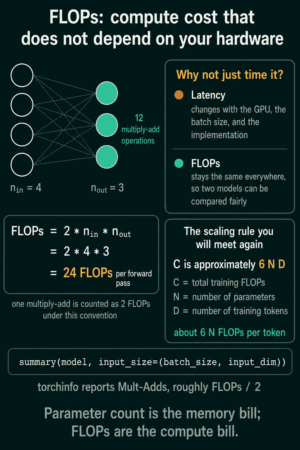
A FLOP is one floating point operation, such as one multiplication or one addition. The FLOPs of one forward pass measure compute cost independent of hardware, so two models can be compared fairly, while timings change with the GPU, the batch size, and the code.

Each output of a linear layer is a dot product over $n_{\text{in}}$ inputs, which takes $n_{\text{in}}$ multiply-adds (multiply one input by its weight, add it to a running sum). Counting each multiply-add as 2 FLOPs:

$$\text{FLOPs} = 2 \times n_{\text{in}} \times n_{\text{out}}$$

So a layer with 4 inputs and 3 outputs does 12 multiply-adds, or 24 FLOPs per example. The cost grows with the batch: a batch of 32 examples takes 32 times the FLOPs of one.

1import torch.nn as nn
2 
3model = nn.Sequential(nn.Linear(784, 256), nn.ReLU(), nn.Linear(256, 10))
4 
5def linear_flops(model, batch_size=1):
6    """FLOPs of the Linear layers in one forward pass, 2 per multiply-add."""
7    total = 0
8    for m in model.modules():
9        if isinstance(m, nn.Linear):
10            total += 2 * m.in_features * m.out_features * batch_size
11    return total
12 
13print(f"batch 1:  {linear_flops(model):,} FLOPs")
14print(f"batch 32: {linear_flops(model, batch_size=32):,} FLOPs")

1batch 1:  406,528 FLOPs
2batch 32: 13,008,896 FLOPs

The formula leaves out the bias additions and the ReLU, which are small next to the multiply-adds. For larger models, the torchinfo package prints a per-layer summary with summary(model, input_size=(batch_size, input_dim)), and its "Mult-Adds" total is roughly FLOPs divided by 2.

FLOPs also connect to parameter count. Training a transformer takes about $6N$ FLOPs per training token, where $N$ is the number of parameters. Over $D$ training tokens, the total training compute $C$ is:

$$C \approx 6ND$$

This is the relationship used to plan large language model pretraining.

A 4-input, 3-output layer doing 12 multiply-adds, FLOPs = 2 x 4 x 3 = 24 per forward pass, why FLOPs compare fairly across hardware while latency does not, the C ≈ 6ND training rule, and the torchinfo summary call that reports Mult-Adds

Latency

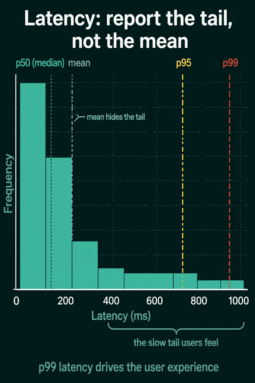
Latency is the time from receiving a request to returning the result, which is what a user waits through. Latency varies from one request to the next, so it is reported as a distribution rather than one number. The mean hides the slow requests, so latency is usually reported as percentiles:

p50 (the median): half of the requests are faster.
p95: 95% of requests are faster.
p99: 99% of requests are faster, a common number to plan a service around.

The slow end, called the tail, is what users feel. A user who triggers 100 calls waits for the slowest of them, so an app that makes many model calls per page is limited by its p99.

1import time
2import torch
3import torch.nn as nn
4 
5torch.manual_seed(0)
6model = nn.Sequential(nn.Linear(784, 256), nn.ReLU(), nn.Linear(256, 10))
7model.eval()
8test_data = [torch.randn(1, 784) for _ in range(1000)]
9 
10latencies = []
11with torch.no_grad():
12    for x in test_data[:20]:          # warm-up, results thrown away
13        _ = model(x)
14    for x in test_data:
15        start = time.perf_counter()
16        _ = model(x)
17        latencies.append(time.perf_counter() - start)
18 
19ms = torch.tensor(latencies) * 1000
20print(f"mean: {ms.mean():.3f}ms")
21for q in (50, 95, 99):
22    print(f"p{q}: {torch.quantile(ms, q / 100):.3f}ms")

One run on a laptop CPU printed:

1mean: 0.108ms
2p50: 0.073ms
3p95: 0.248ms
4p99: 0.581ms

Numbers vary by run and machine. In this run p99 is about 8 times the median, and the mean of 0.108 ms says little about either. The warm-up calls are thrown away because they pay one-time costs such as memory allocation. On a GPU, add torch.cuda.synchronize() after the warm-up and after each model(x). GPU work is queued, so without the sync the timer measures submission, not the computation.

A right-skewed latency histogram with dashed lines for the median, the mean, p95, and p99, showing the slow tail users feel to the right of the mean

Throughput

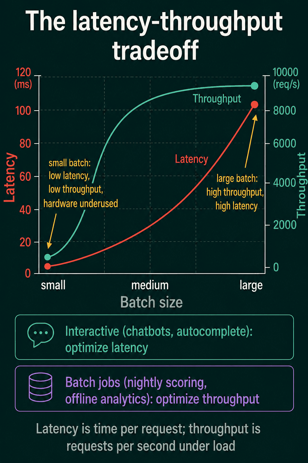
Throughput is how many examples the model processes per second under load. Batch size trades it against latency. A batch of 1 has low latency but leaves the hardware mostly idle. A large batch keeps it busy and raises throughput, but each request waits for the whole batch.

1import time
2import torch
3import torch.nn as nn
4 
5torch.manual_seed(0)
6model = nn.Sequential(nn.Linear(784, 256), nn.ReLU(), nn.Linear(256, 10))
7model.eval()
8 
9def time_batch(batch_size, repeats=200):
10    """Median seconds for one forward pass over a batch of this size."""
11    x = torch.randn(batch_size, 784)
12    times = []
13    with torch.no_grad():
14        for _ in range(20):           # warm-up
15            model(x)
16        for _ in range(repeats):
17            start = time.perf_counter()
18            model(x)
19            times.append(time.perf_counter() - start)
20    return torch.tensor(times).median().item()
21 
22for batch_size in (1, 32, 256):
23    t = time_batch(batch_size)
24    print(f"batch {batch_size:>3}: latency {t * 1000:.3f}ms, "
25          f"throughput {batch_size / t:,.0f} examples/sec")

1batch   1: latency 0.066ms, throughput 15,201 examples/sec
2batch  32: latency 0.164ms, throughput 195,470 examples/sec
3batch 256: latency 0.702ms, throughput 364,712 examples/sec

In this run, going from a batch of 1 to a batch of 256 made each batch about 11 times slower and raised throughput about 24 times. Interactive apps such as chatbots and autocomplete should optimize latency, since a person is waiting. Batch jobs such as nightly scoring or offline analytics should optimize throughput, since only the total time counts.

Latency and throughput rising with batch size, with interactive apps marked optimize latency and batch jobs marked optimize throughput

Model size: memory footprint

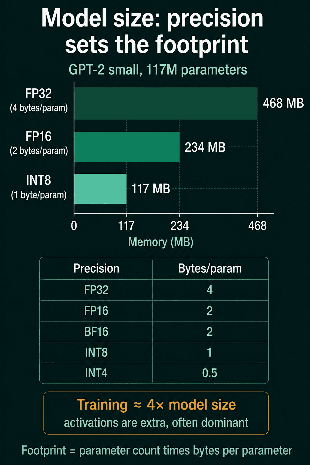
A model's memory footprint is its parameter count times the bytes used to store each parameter, which is set by the precision, the number format of each value:

Precision	Bytes per parameter
FP32 (float32)	`4`
FP16 (float16)	`2`
BF16 (bfloat16)	`2`
INT8	`1`
INT4	`0.5`

GPT-2 small, with 117 million parameters, takes $117 \times 10^6 \times 4 = 468$ MB in FP32, 234 MB in FP16, and 117 MB in INT8. In PyTorch, p.element_size() returns the bytes per element of a tensor:

1import torch.nn as nn
2 
3model = nn.Sequential(nn.Linear(784, 256), nn.ReLU(), nn.Linear(256, 10))
4 
5def size_mb(model):
6    """Bytes taken by the parameters, in megabytes."""
7    return sum(p.numel() * p.element_size() for p in model.parameters()) / 1e6
8 
9print(f"FP32: {size_mb(model):.3f} MB")
10model.half()                      # cast every parameter to FP16
11print(f"FP16: {size_mb(model):.3f} MB")

1FP32: 0.814 MB
2FP16: 0.407 MB

Training also stores one gradient per parameter, the same size as the model again, and the Adam optimizer keeps two running averages per parameter, twice the model size. Weights, gradients, and optimizer states in FP32 come to about 4 times the model size. Activations, the intermediate outputs of each layer saved for the backward pass, are a separate pool on top of that, often the largest part at large batch sizes. Activation checkpointing, which recomputes some activations in the backward pass instead of storing them, shrinks that pool and leaves the 4 times untouched.

GPT-2 small taking 468 MB in FP32, 234 MB in FP16, and 117 MB in INT8, a bytes-per-parameter table, and a note that training takes about 4 times the model size plus activations

Which number to check, and common mistakes

Start from where the model runs: model size for a phone or a small GPU, p95 and p99 for a user-facing service, throughput for a large offline job. FLOPs and parameter count are for comparing models across hardware or before training.

Reporting mean latency. The mean can look fine while 1 request in 100 takes several times longer.
Timing without warm-up, or without a GPU sync. Without them, the timer measures setup costs and queueing.
Reading parameter count as speed. A sparse model can have more parameters and still run faster than a dense one.
Budgeting training memory from the weights alone. Gradients and Adam's two averages bring it to about 4 times the weights before any activations.

Picking the quality metric is covered in how to choose an evaluation metric. Why Adam keeps two running averages per parameter is explained in the Adam optimizer post.

QuiddityML teaches each of these five measurements as its own concept in the ML Foundation track, and the exercises on them include counting the FLOPs of an nn.Linear(512, 256) layer step by step, working out throughput at two batch sizes from their timings, and adding up the training memory of a 350M-parameter model under Adam.